Introduction #
We now move on to consider the valuation of payments which are not certain – payments which have a probability of occurrence which is not necessarily 1.
For example:
- General Insurance – claim size, number of claims per policy.
- Life Insurance – when will the policyholder die? How many premiums will be paid?
- Life annuity – how long the policyholder will survive?
- Coupon bonds – will the borrower default?
EPV of a single contingent payment #
Contingent payment #
If a payment under an insurance policy, or any other financial transaction, depends on the occurrence of a certain event (e.g. a person dying within a given period, or a person surviving a given period), we call such an event a contingent event.
The corresponding payment is referred to as a contingent payment.
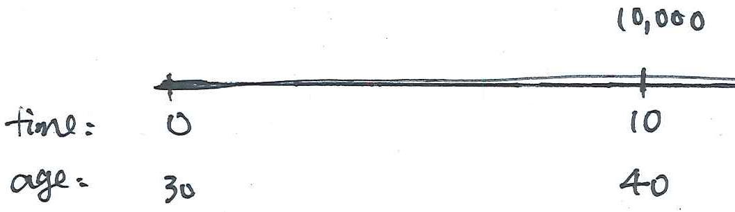
Example: pure endowment #
In a pure endowment insurance, if the policyholder aged (30) survives 10 years, then the insurance benefit of $10,000 payable at time \(10\). Assume an interest rate of 6% per annum effective.
Find an expression for the EPV of this survival benefit.
Principle of equivalence #
If a premium is calculated according to the principle of equivalence, then the expected present value of premium income equals the expected present value of the benefits under the policy.
The premium obtained using this principle is sometimes referred to as a pure premium. This is the pure expected value of the benefit, before any adjustment is made (e.g. market adjustments, risk loading, ).
Example 1 #
Suppose that an insurance contract pays $10,000 at two possible times in the future.
In particular, there is a 40% chance that the payment will have to be made in 5 years’ time and there is a 60% chance that the payment will have to be made in 10 years’ time.
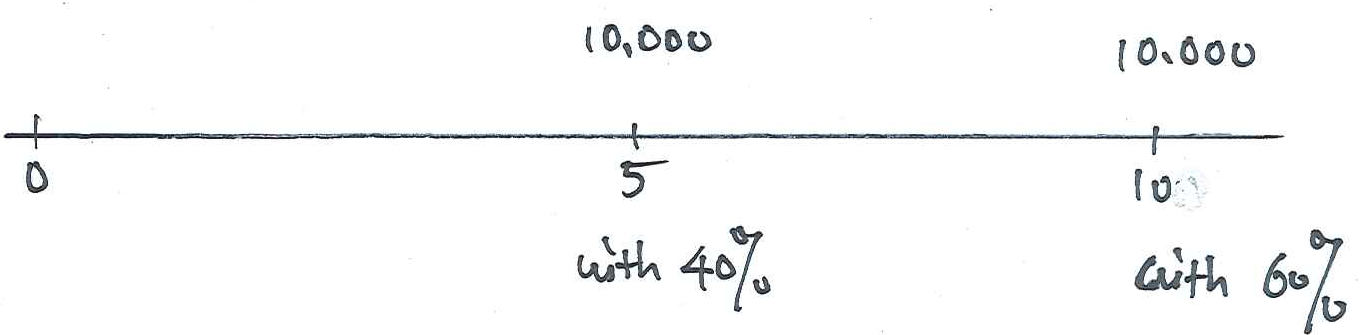
Assuming an interest rate of 6% per annum effective, calculate the EPV of the required insurance benefit.
Solution #
The present value of the required payment is clearly uncertain. This present value, denoted PV, is a random variable that can take two distinct values depending on the timing of the $10,000 payment.
The values that the random variable PV can take are:
\(10,\!000 \times 1.06^{-5}\)with probability\(0.4\)\(10,\!000 \times 1.06^{-10}\)with probability\(0.6\)
The expected value of the PV is therefore
\begin{eqnarray*} \text{EPV}=E[\text{PV}] &=&0.4\times 10,000\times 1.06^{-5} \\ &&+0.6\times 10,000\times 1.06^{-10} =\$6,\!339.40. \end{eqnarray*}
The EPV is the pure premium for this insurance contract.
Analysis of Example 1 #
Suppose that the insurer sets aside the EPV=$6,339.40 (pure premium income) to fund the future payment.
At 6% per annum effective, the accumulation of the EPV over 5 years
is
\begin{equation*} 6,\!339.40\,(1.06^{5})=8,\!483.55 \end{equation*}
and the accumulation of the EPV over 10 years is
\begin{equation*} 6,\!339.40\,(1.06^{10})=11,\!352.90. \end{equation*}
Thus, if the payment of $10,000 is due in 10 years, we would have sufficient funds to make the payment, whereas if it were due in 5 years, we would not.
Is this an issue?
Suppose now that there were 1,000 such contracts (all mutually independent):
- for each contract the probability that the payment is due in 5 years’ time is 0.4, and the probability that the payment is due in 10 years’ time is 0.6.
- the total pure premium income for the 1000 contracts is
\begin{equation*} 6,\!339.40\times 1,\!000= 400\times 10,\!000\times 1.06^{-5}+600\times 10,\!000\times 1.06^{-10}. \end{equation*} - among those 1,000 contracts, we expect 40% of the contracts to require a payment of $10,000 at time 5 years, and 60% to require a payment at time 10 years.
-
after 5 years we expect to have
\begin{equation*} 1000\times 6,\!339.40\times 1.06^{5}-400\times 10,\!000=4,\!483,\!547.2 \end{equation*} -
after 10 years we expect to have $$ \left( 1000\times 6,339.40\times 1.06^{5}-400\times 10,000\right) \times 1.06^{5}-600\times 10,000 $$ which is the same as
\begin{eqnarray*} &&1.06^{10}\big(1,\!000\times 6,\!339.40-400\times 10,\!000\times 1.06^{-5} \\ &&\hspace{1.5in}-600\times 10,\!000\times 1.06^{-10}\big)\\ &=&1.06^{10}\times 1,\!000\times \big( 6,\!339.40-0.4\times 10,000\times 1.06^{-5} \\ &&\hspace{1.5in}-0.6\times 10,\!000\times 1.06^{-10}\big)=0. \end{eqnarray*}
Note:
- of course the 40% and 60% are probabilities, and the actual, proportions may not be exactly the same. This is why some margin may have to be added to the pure premium, to guarantee all payments to a certain level of confidence.
- if one focussed exclusively on this randomness, how much would the insurance company need to be 100% certain of having enough money?
- additionally, typically, the interest rate would also be uncertain, and there would be additional uncertainties to take into account as well.
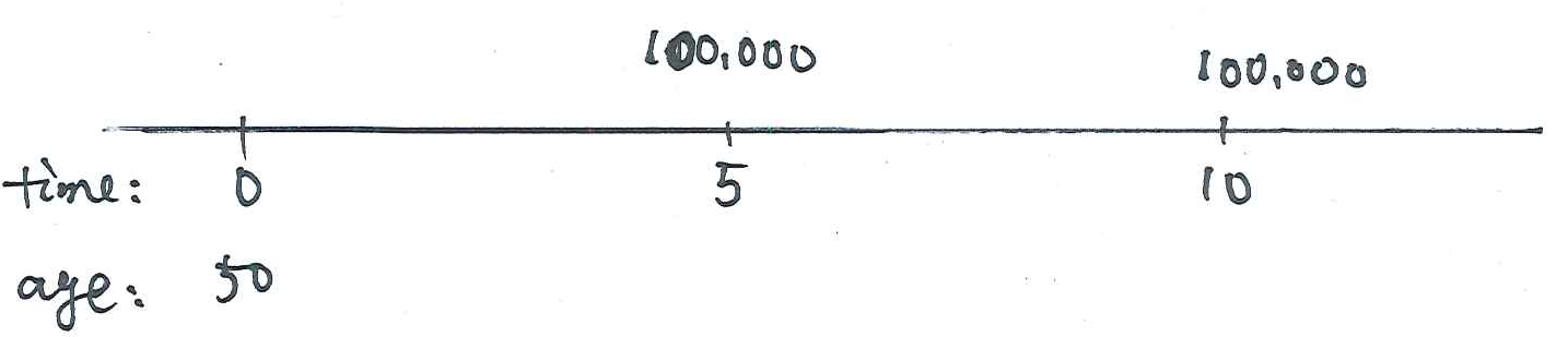
Example 2 #
Consider an insurance policy which is sold to a female currently aged 50. The benefits under this insurance policy are:
- if she dies within five years, her estate is paid $100,000 after five years;
- if she dies no earlier than five years but no later than ten years, then her estate is paid $100,000 after ten years;
- nothing is paid to her estate (or her) if she survives to age 60.
- The effective rate of interest per annum is 6%. Assume the mortality of this female follows the Female Mortality Table in the tutorial book.
Calculate the EPV of the benefits paid under this insurance policy.
Solution #
We create a table of present values and their associated probabilities as follows:
| Present Value | Probability |
|---|---|
\(100,\!000\times 1.06^{-5}\) |
\((l_{50}-l_{55})/l_{50}\) |
\(100,\!000\times 1.06^{-10}\) |
\((l_{55}-l_{60})/l_{50}\) |
\(0\) |
\(l_{60}/l_{50}\) |
Thus, the EPV is
\begin{eqnarray*} &&100,\!000\times 1.06^{-5}\ \frac{94,\!692-92,\!349}{94,\!692} \\ &+&100,\!000\times 1.06^{-10}\ \frac{92,\!349-88,\!703}{94,\!692} \\ &=&\$3,\!999. \end{eqnarray*}
EPV of a series of contingent payments #
Introduction #
- Previously we considered the calculation of the EPV of a single payment made (perhaps) at some (possibly random) time in the future.
- In Example 1, we found the EPV of a payment which was made (or not made) depending on the time of death of a life aged 50.
- We now consider payments which are made if and only if a condition is realised at particular times.
- It is clear that this could be considered as “being alive” and/or “being dead,” leading to the context of life insurance products, but the formulas are general and apply to any such contingent event.
- We thus generalise results to multiple possible (contingent) payments.
A life insurance example #
- Consider a life aged 30.
- Consider also a series of payments made at times 1, 2 and 3.
- These payments are made only if the life currently aged 30 is alive at those times.
- Determine an expression for the EPV of the payments made under this agreement.
- Note this is a term life annuity which we will denote
$$a_{30:\angl{3}}.$$
Considering all possible outcomes (either/or) of present values PV (a random variable):
| Event | Present Value (PV) | Probability |
|---|---|---|
\((30)\) dies during period [0,1) |
0 | \(q_{30}\) |
\((30)\) dies during period [1,2) |
\(a_{\angl{1}}\) |
\(p_{30}- {_2 p}_{30}\) |
\((30)\) dies during period [2,3) |
\(a_{\angl{2}}\) |
\({_2 p}_{30} - {_3 p}_{30}\) |
\((30)\) survives to time 3 |
\(a_{\angl{3}}\) |
\({_3 p}_{30}\) |
Hence the expectation of the PV, the “EPV” of the series of payments is
\begin{eqnarray*} \text{EPV}&=&a_{\angl{1}}\,(p_{30}-{}_2p_{30}) +a_{\angl{2}}\,({}_2p_{30}-{}_3p_{30}) +a_{\angl{3}}\times {}_3p_{30}\qquad\quad\\ &=&v (p_{30}-{}_2p_{30}) +(v+v^2)({}_2p_{30}-{}_3p_{30})+(v+v^2+v^3)\times {}_3p_{30}\\ &=&v p_{30}+v^2 {}_2p_{30}+v^3 {}_3p_{30} \end{eqnarray*}
Note:
- The EPV of the three contingent payments is the sum of the EPV of each of the three individual continent payments.
- This is crucial, because this gives us two different ways of calculating the EPV:
- Calculate a weighted average of the PV’s, with weights being the associated probabilities. This is the first line in the equation above.
- Calculate a weighted average of the present value of individual cash flows, weighted by their associated probabilities of occurence. This is the last line in the equation above.
Preliminary: changing the order of summation #
Because of the alternative ways of calculating the EPV as discussed above, we may need to swap summations to move from one case to the other.
Consider $$\sum_{k=1}^{n}\sum_{j=1}^{k}a_{k,j}\text{ .} $$
This can be written as
\begin{eqnarray*} &&a_{1,1}+ \\ &&a_{2,1}+a_{2,2}+ \\ &&a_{3,1}+a_{3,2}+a_{3,3}+ \\ &&\ldots \\ &&a_{n,1}+a_{n,2}+a_{n,3}+\ldots +a_{n,n} \end{eqnarray*}
The sum of the first column is \(\sum_{k=1}^{n}a_{k,1}\) , the sum of the second is \(\sum_{k=2}^{n}a_{k,2}\) , and so on until the sum of the last column is \(\sum_{k=n}^{n}a_{k,n}=a_{n,n}\).
Thus
\begin{eqnarray*} \sum_{k=1}^{n}\sum_{j=1}^{k}a_{k,j} &=&\sum_{k=1}^{n}a_{k,1}+\sum_{k=2}^{n}a_{k,2}+\ldots +\sum_{k=n}^{n}a_{k,n}\\ && \\ &=&\sum_{j=1}^{n}\sum_{k=j}^{n}a_{k,j}\text{.} \end{eqnarray*}
The EPV of a series of payments – general case #
- We now consider the more general case of the above example
- We noted that the EPV of a series of payments is equal to the sum of the EPVs of each of the payments in the series.
- We will assume the following:
- Suppose we have a series of payments made at times
\(1,2,\ldots ,n\). - These payments are denoted
\(X_{1},X_{2},\ldots ,X_{n}\). - The present value of the first
\(k\)payments is denoted\(V_{k}\)such that$$V_{k}=\sum_{j=1}^{k}v^{j}X_{j}.$$ - The payment at time
\(t\)can be made only if all previous payments have been made. In other words, what is random is when the payment will stop (the final\(k\)in the expression above).
- Suppose we have a series of payments made at times
Of course these are quite restrictive assumptions (especially the last one), but we focus on this for now as it simplifies calculations and it ties in
well with the life insurance applications.
Necessary probabilities #
- Let
\(p_{k}\)be the probability that at least\(k\)payments are made. - We define
\(\pi _{k}\)to be the probability that exactly\(k\)payments are made. - Then we have the following relationship between
\(\{p_k\}_{k=1}^n\)and\(\{\pi_k\}_{k=1}^n\):\begin{eqnarray*} \pi_1&=&p_1-p_2,\\ \pi_2&=&p_2-p_3,\qquad\qquad\qquad\qquad\qquad\qquad\qquad\qquad\\ \vdots&=& \vdots\\ \pi_k&=&p_k-p_{k+1},\\ \vdots &=& \vdots\\ \pi_{n-1}&=&p_{n-1}-p_n,\\ \pi_n&=&p_n. \end{eqnarray*}
Someone with a sharp eye will recognise differences of probabilities
seen earlier.
The EPV of a series of payments #
Then we have $$p_{k}=\sum_{j=k}^{n}\pi _{j}. $$
The EPV of the series of \(n\) payments is
\begin{eqnarray*} \sum_{k=1}^{n}\pi _{k}V_{k} &=&\sum_{k=1}^{n}\sum_{j=1}^{k}\pi _{k}v^{j}X_{j} \\ &=&\sum_{j=1}^{n}\sum_{k=j}^{n}\pi _{k}v^{j}X_{j} \qquad\qquad\qquad\qquad\qquad\qquad\qquad\qquad\\ &=&\sum_{j=1}^{n}v^{j}X_{j}\sum_{k=j}^{n}\pi _{k} =\sum_{j=1}^{n}v^{j}X_{j}p_{j}. \end{eqnarray*}
This proves that the EPV of a series of payments can here be
calculated as the sum of the EPVs of each payment in the series.
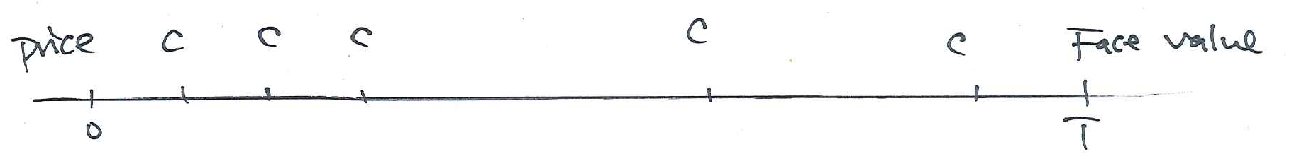
Example: Fixed Coupon Bond subject to Default #
- Suppose that a corporation issues a bond to the public.
- The bond’s face value is $100.
- The bond has 4 years until maturity and will pay coupons of 7% per annum, payable half yearly.
- Find the price of the bond assuming a yield of 8% per annum convertible half yearly.
- Assume that the probability that the corporation will be able to make the payment in
\(t\)half years is\(p_t=0.99^{t}\).
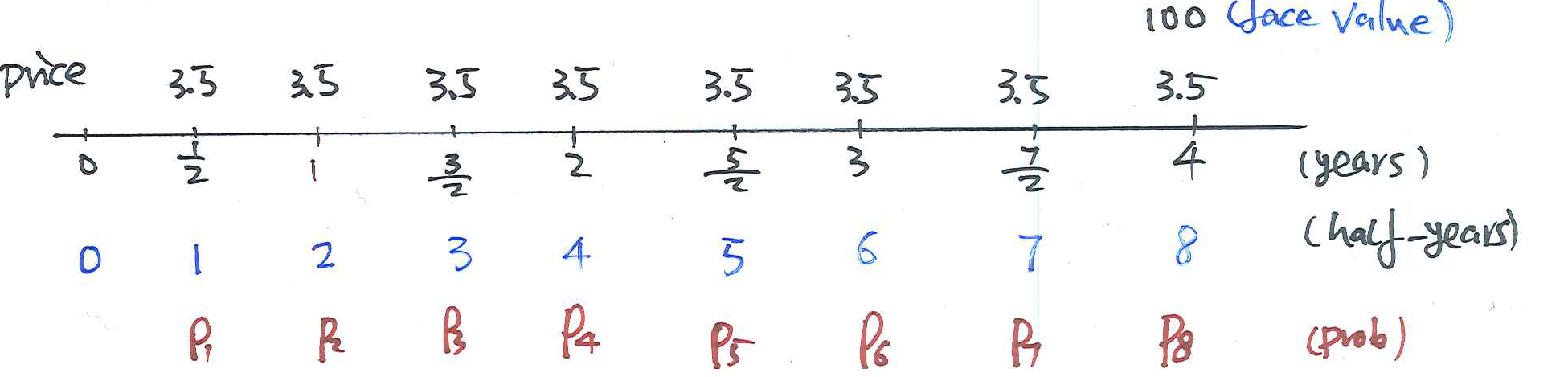
The price of this defaultable bond is the EPV of the coupon payments and the face value.
\begin{eqnarray*} \text{Price}&=&\sum_{t=1}^8 3.5\times (1.04)^{-t}\times 0.99^t+100 \times (1.04)^{-8} \times 0.99^8\\ &=&3.5\sum_{t=1}^8 \left(\frac{0.99}{1.04}\right)^t+100\times \left(\frac{0.99}{1.04}\right)^8, \qquad\qquad \frac{0.99}{1.04}=\frac{1}{1+j}\\ &=&3.5\sum_{t=1}^8 \left(\frac{1}{1+j}\right)^t+100\times \left(\frac{1}{1+j}\right)^8, \qquad \qquad j=0.0505\\ &=&3.5 a_{\angl{8}}@j+100\times \left(\frac{1}{1+j}\right)^8=3.5\times 6.450+67.4242=90\,. \end{eqnarray*}
Life insurance premium calculations #
Introductory example #
Term insurance benefits #
Recall the insurance policy we considered in Example 2. From that exercise, we had:
- a sum insured of $100,000
- the life insured is a 50 year old female
- there is payment
- after 5 years if (50) dies in the first five years (before 55)
- after 10 years if (50) dies between times five years and ten years (between 55 and 60)
- no payment otherwise
- effective rate of interest was 6% per annum
- EPV of death benefit = $3,999
Annual premiums and the equation of value #
- Consider now the case where premiums for this insurance contract are paid annually in advance while (50) is alive but for a maximum of three years.
- What is the fair annual premium
\(P\)? - To solve for annual premium
\(P\), we use the “equation of value”$$\text{EPV of the premiums} = \text{EPV of the death benefit}.$$ - Thus
\begin{equation*} 3,\!999=P\left( 1+vp_{50}+v^{2}\ _{2}p_{50}\right) \end{equation*}with\(p_{50}=l_{51}/l_{50}=0.99590\)and\(_{2}p_{50}=l_{52}/l_{50}=0.99141.\) - Finally,
\begin{equation*} 3,\!999=2.82188P \end{equation*}giving $P=$1,!417$ to the nearest dollar.
General assumptions / notation #
- we generally assume that the death benefit is payable at the end of the year of death
- we generally assume that the annual premium is payable in advance
- let
\(S\)be the sum insured - premiums are calculated using the principle of equivalence
EPV of life insurance contracts #
Definitions #
Whole life Insurance:
- insurance contract that will pay an amount of money (the sum insured) on the death, whenever that might be, of a life
currently aged
\(x\) - EPV of such a contract with sum insured $1 is denoted
$$A_{x}$$
Term life insurance:
- insurance contract that will pay an amount of money (the sum insured) on the death, provided this occurs before
\(n\)years, of a life currently aged\(x\) - EPV of such a contract with sum insured $1 is denoted
$$A_{x:\angl{n}}^{1}$$
EPV of \(A_x\)
#
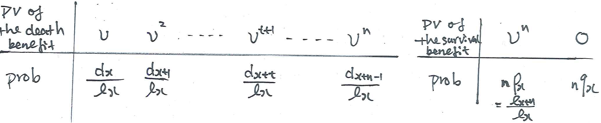
A payment of $1 is made at the end of the year of death:
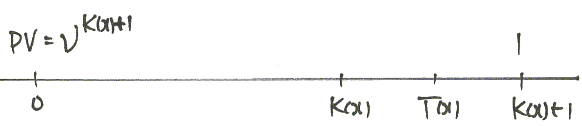
Recall
\begin{eqnarray*} \Pr[K(x)=t]&=&\Pr[t\le T(x)<t+1]=\ _tp_x-\ _{t+1}p_x\\ &=&\frac{l_{x+t}}{l_x}-\frac{l_{x+t+1}}{l_x} =\frac{d_{x+t}}{l_x}, \quad t=0, 1, 2, \ldots. \end{eqnarray*}
The PV of the death benefit is \(v^{K_x+1}\) which follows the distribution:
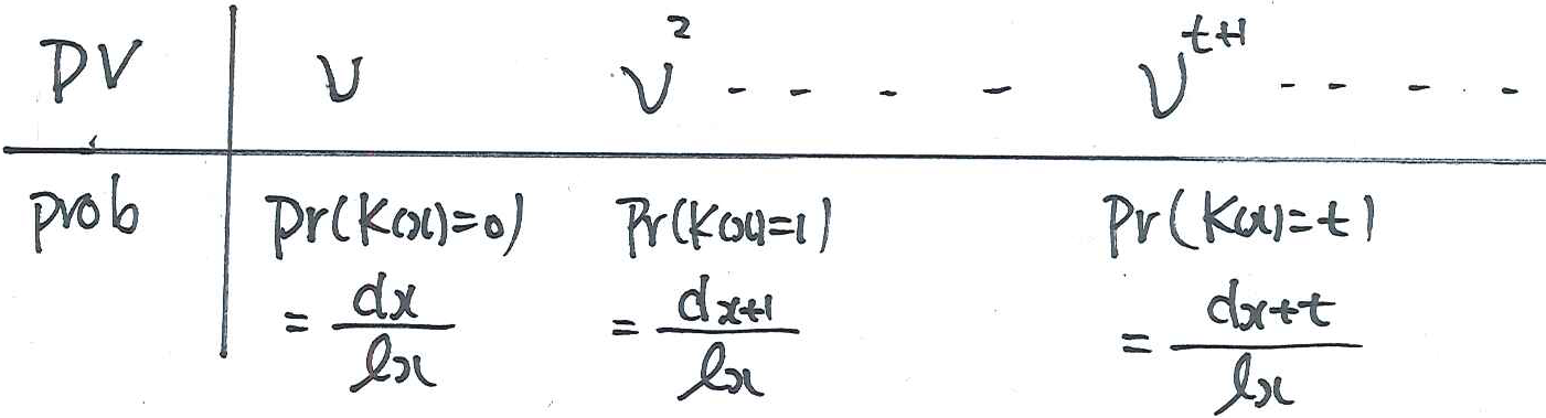
The expected present value (EPV) of the death benefit becomes then $$A_{x}=\sum_{t=0}^{\infty }v^{t+1},\frac{d_{x+t}}{l_{x}}. $$
This can easily be calculated using a spreadsheet. For
example, to compute \(A_{60}\) when \(i=0.05\) from the set of values \(l_{60},l_{61},l_{62},...\), we would set up columns like:
\(t\) |
\(l_{60+t}\) |
\(v^{t+1}\) |
\(d_{60+t}/l_{60}\) |
Product |
|---|---|---|---|---|
| 0 | 79,062 | 0.9524 | 0.0209 | 00199 |
| 1 | 77,411 | 0.9070 | 0.0224 | 0.0204 |
| 2 | 75,637 | 0.8638 | 0.0241 | 0.0208 |
| … | … | … | … | … |
\(w-60\) |
\(l_w\) |
\(v^{w-60+1}\) |
\(d_w/l_{60}\) |
where \(w\) is the final age of a life table.
The sum of the terms in the ‘Product’ column gives the value of \(A_{60}\).
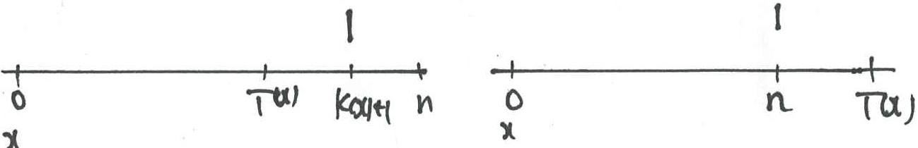
EPV of \(A_{x:\angl{n}}^{1}\)
#
For a term life insurance, simply stop the sum after \(n\) years rather than running the sum all the way to \(\omega\).
Also,
$$A_{x:\angl{n}}^{1} = A_x - \frac{l_{x+n}}{l_n}v^n A_{x+n}.$$
This is analogous to the formula
$$a_{\angl{n}}=a_\infty - v^n a_\infty,$$
but taking probability of death (contingencies) on top.
EPV of endowments #
Definitions #
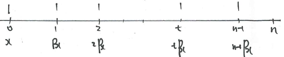
Pure Endowment:
- insurance contract that will pay an amount of money (the sum insured) after
\(n\)years, provided its insured life, currently aged\(x\), has survived those\(n\)years. - EPV of such a contract with sum insured $1 is denoted
$$A_{x:\angl{n}}^{\,\,\,\,1}$$
Endowment:
- insurance contract that will pay an amount of money (the sum insured) on the death of a life currently aged
\(x\)if this happens before\(n\)years, or in exactly\(n\)years if the insured has survived that time. - EPV of such a contract with sum insured $1 is denoted
$$A_{x:\angl{n}}=A_{x:\angl{n}}^{1}+A_{x:\angl{n}}^{\,\,\,\,1}$$
EPV of \(A_{x:\angl{n}}^{\,\,\,\,1}\) and \(A_{x:\angl{n}}\) and
#
\(A_{x:\angl{n}}\) is the EPV of a benefit of 1 payable at the end of the
year of death of a life now aged \(x\), if this occurs within \(n\) years, or at
time \(n\) if \((x)\) survives for \(n\) years.
$$A_{x:\angl{n}}=A_{x:\angl{n}}^{1}+A_{x:\angl{n}}^{\,\,\,\,1}$$
- We know how to calculate the left hand side
\(A_{x:\angl{n}}^{1}\). - The right hand side is simply
$$A_{x:\angl{n}}^{\,\,\,\,1}=v^n {_t p}_x.$$
Hence, to calculate \(A_{x:\angl{n}}\), we use
$$A_{x:\angl{n}}=\sum_{t=0}^{n-1}v^{t+1}\,\frac{d_{x+t}}{l_{x}}+v^{n}\,_{n}p_{x} = A_{x:\angl{n}}^{1}+A_{x:\angl{n}}^{\,\,\,\,1}$$
Note:
- If
\(n=1\), then\(A_{x:\angl{1}}^{1}= vq_x\)and\(A_{x:\angl{1}}=v(q_x+p_x)=v\)(payment at time 1 is certain) - If
\(n\)goes to\(\infty\), then $$ \lim_{n\to\infty} A_{x:\angl{n}}^{1}=A_x,;\lim_{n\to\infty} A_{x:\angl{n}}^{,,,,1}=0,;\Longrightarrow ; \lim_{n\to\infty} A_{x:\angl{n}}=A_x$$
EPV of life annuities #
Definitions #
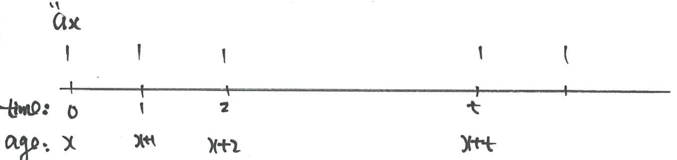
Life annuity:
- insurance contract that will pay an amount of money (the sum insured) every year for as long as the insured, currently aged
\(x\), survives. - if payments are made at the end of each year (that is, payments start in 1 year), this is denoted
$$a_x$$ - if payments are made at the beginning of each year (that is, payments start immediately), this is denoted
$$\ddot{a}_x$$ - these notations are for payments of $1 p.a., as usual.
Term life annuity
- insurance contract that will pay an amount of money (the sum insured) every year for as long as the insured, currently aged
\(x\), survives, but no longer than\(n\)years. - if payments are made at the end of each year (that is, payments start in 1 year), this is denoted
$$a_{x:\angl{n}}$$ - if payments are made at the beginning of each year (that is, payments start immediately), this is denoted
$$\ddot{a}_{x:\angl{n}}$$ - these notations are for payments of $1 p.a., as usual.
EPV of life annuities #
Using the result that the EPV of a series of payments is the sum of the EPVs
of each payment in the series, we have
$$\ddot{a}_{x}=\sum_{t=0}^{\infty }v^{t}\ _{t}p_{x}.$$
To calculate \(\ddot{a}_{x:\angl{n}}\), we use
$$\ddot{a}_{x:\angl{n}}=\sum_{t=0}^{n-1}v^{t\,}\,_{t}p_{x}$$
Such calculations can easily be performed using a spreadsheet.
For example, to compute \(\ddot{a}_{60}\) at \(i=0.05\) from the set of
values \(l_{60},l_{61},l_{62},...\), we would set up columns like:
\(t\) |
\(l_{60+t}\) |
\(v^{t}\) |
\(_{t}p_{60}\) |
Product |
|---|---|---|---|---|
| 0 | 79,062 | 1.0000 | 1 | 1 |
| 1 | 77,411 | 0.9524 | 0.97911 | 0.93249 |
| 2 | 75,637 | 0.9070 | 0.95668 | 0.86773 |
| … | … | … | … | … |
\(w-60\) |
\(l_w\) |
\(v^{w-60}\) |
\(_{w-60}p_{60}\) |
|
\(\ddot{a}_{60}=\)Sum |
where \(w\) is the final age of a life table. In ALT 2000-2002, \(w=110.\)
As for the life insurance table, the desired result \((\ddot{a}_{60})\) is the sum of the values in the “Product” column.
Calculating insurance premiums #
Typical assumptions #
Typically, premiums are paid
- in advance
- for life or up to
\(n\)years - in the latter case, we can distinguish two scenarios:
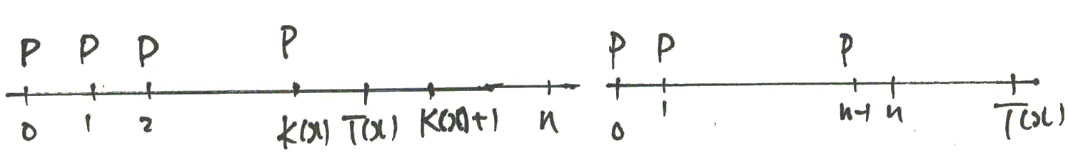
Hence, the EPV of premiums needs to be calculated with the help of life annuities, as the number of payments is uncertain and depends on survival of the insured.
Principle of equivalence #
Recall that the principle of equivalence requires $$\text{EPV Premiums} = \text{EPV Benefits}. $$ The EPV of premiums will be
\(P \ddot{a}_{x:\angl{n}}\)in case of\(n\)year payment period\(P \ddot{a}_x\)potentially, but only in case of whole life payments (people would not pay premiums beyond their coverage period)
The EPV of benefits will be simply
\begin{eqnarray*} S \cdot A_x && \text{in case of whole life insurance}, \\ S \cdot A_{x:\angl{n}}^{1} && \text{in case of term life insurance}, \\ S \cdot A_{x:\angl{n}}^{\,\,\,\,1}&& \text{in case of pure endowment}, \\ S \cdot A_{x:\angl{n}}&& \text{in case of endowment} . \end{eqnarray*}
Example 3 #
An endowment insurance with a term of 3 years is sold to a life currently aged 45.
The sum insured is $10,000. Premiums are payable annually in advance while the life is alive for a maximum of three years.
Assume an interest rate of 6% per annum effective in your calculations.
Using the mortality rates from the Male Mortality Table in Atkinson and Dickson (2011) (also in the Tutorial book), calculate the actuarially fair annual premium.
We use the principle of equivalence to get
\begin{equation*} P \ddot{a}_{45:\angl{3}} = 10,\!000 A_{45:\angl{3}}$$
We have $$\ddot{a}{45:\angl{3}}=1+v,p{45}+v^{2} ,{2}p{45}=2.8191
\end{equation*}and $$A_{45:} =( v,d_{45}+v{2},d_{46}+v{3},d_{47}+v^{3},l_{48}) = 0.840428.$$Substituting, we finally obtain`
Relationships between actuarial functions #
Introduction #
Recall that we were able to derive identities and relationships in the context of time value of money.
For instance, we showed that
$$\ddot{a}_{\angl{n}}= 1+ a_{\angl{n-1}}$$
Can we derive similar relationships in the context of life annuities?
Recursive formula for \(\ddot{a}_{x}\)
#
We have
$$\ddot{a}_{x}=1+vp_{x}\ \ddot{a}_{x+1}$$
Interpretation:
Proof:
Starting with the LHS, we have
\begin{eqnarray*} \ddot{a}_{x} &=&\sum_{t=0}^{\infty }v^{t}\,_{t}p_{x}=1+\sum_{t=1}^{\infty }v^{t}\,_{t}p_{x} \\ && \\ &=& 1+\sum_{r=0}^{\infty }v^{r+1}\,_{r+1}p_{x} \\ && \\ &=& 1+v\,\sum_{r=0}^{\infty }v^{r}\,p_{x}\,_{r}p_{x+1} \\ && \\ &=& 1+v\,p_{x}\,\sum_{r=0}^{\infty }v^{r}\,_{r}p_{x+1} \\ && \\ &=& 1+v\,p_{x}\,\ddot{a}_{x+1} \end{eqnarray*}
Relationship between \(A_{x:\angl{n}}\) and \(\ddot{a}_{x:\angl{n}}\)
#
One can show that the two following identities hold:
\begin{eqnarray*} A_{x:\angl{n}}+(1-v)\ddot{a}_{x:\angl{n}}&=&1,\\ &&\\ A_{x}+(1-v)\ddot{a}_{x}&=&1. \end{eqnarray*}
Proof #
We have
$$A_{x:\angl{n}}+(1-v)\ddot{a}_{x:\angl{n}}\hspace{3in} $$
\begin{eqnarray*} &=& \sum_{t=0}^{n-1}v^{t+1}\,\frac{d_{x+t}}{l_{x}}+v^{n}\,\frac{l_{x+n}}{l_{x}}+(1-v)\sum_{t=0}^{n-1}v^{t}\,_{t}p_{x} \\ &=& \sum_{t=0}^{n-1}v^{t+1}\,\left( \,_{t}p_{x}-\,_{t+1}p_{x}\right) +v^{n}\,_{n}p_{x}+\sum_{t=0}^{n-1}v^{t}\,_{t}p_{x}-\sum_{t=0}^{n-1}v^{t+1}\,_{t}p_{x} \\ &=& -\sum_{t=1}^{n}v^{t}\,_{t}p_{x}+\sum_{t=0}^{n}v^{t}\,_{t}p_{x}= 1 \end{eqnarray*}
The second case (involving \(A_x\)) is shown in the same way.
Alternative proof using perpetuities #
First, we introduce the effective rate of discount interest \(d\) p.a.. Note that
$$\ddot{a}_{\angl{t}}=(1+i)a_{\angl{t}}=(1+i)\frac{1-v^t}{i}=\frac{1-v^t}{d},$$
where
$$d = \frac{i}{1+i} = 1-v$$
is the discounted amount of \(i\) to time 0. In particular
$$\ddot{a}_{\angl{\infty}}=\frac{1}{d}\quad (=(1+i)a_{\angl{\infty}})$$
and hence it makes sense that
$$\ddot{a}_x=\frac{1-A_x}{d}.$$
This generalises to other cases.
Corollary #
From
$$P\,\ddot{a}_{x:\angl{n}}=S\,A_{x:\angl{n}}$$
we get
$$P=\frac{S\,A_{x:\angl{n}}}{\ddot{a}_{x:\angl{n}}}$$
The equation
$$A_{x:\angl{n}}+(1-v)\ddot{a}_{x:\angl{n}}=1 $$
thus yields
\begin{eqnarray*} P&=&\frac{S\left( 1-(1-v)\ddot{a}_{x:\angl{n}}\right) }{\ddot{a}_{x:\angl{n}}} =S\left( \frac{1}{\ddot{a}_{x:\angl{n}}}-(1-v)\right)\\ &=&(1-v)\frac{S\,A_{x:\angl{n}}}{1-A_{x:\angl{n}}} = d\frac{S\,A_{x:\angl{n}}}{1-A_{x:\angl{n}}} \end{eqnarray*}
Example 4 #
You are given that \(A_{x:\angl{n}}+(1-v)\ddot{a}_{x:\angl{n}}=1\).
Suppose that \(l_{40+t}=95,000-300t\) for \(t=0,1,2,\ldots ,10\).
Compute the annual premium, \(P\), for a 10 year endowment insurance
for a life aged exactly 40 with sum insured $100,000 payable at the end of
the year of death or at maturity using an effective rate of interest of 6%
per annum.
Give your answer to the nearest dollar.
Solution – Premium #
Calculate \(\ddot{a}_{40:\angl{10}}\) first as
\begin{eqnarray*} \ddot{a}_{40:\angl{10}} &=&\sum_{t=0}^{9}v^{t}\,_{t}p_{40}=\sum_{t=0}^{9}v^{t}\,\frac{l_{40+t}}{l_{40}} \\ && \\ &=& \sum_{t=0}^{9}v^{t}\,\frac{95,000-300t}{95,000} \\ && \\ &=& \sum_{t=0}^{9}v^{t}\,\left( 1-\frac{3}{950}t\right) \\ && \\ &=& \ddot{a}_{\angl{10}} -\frac{3}{950}\,\sum_{t=0}^{9}t\,v^{t}\,. \end{eqnarray*}
Now let
$$z=\sum_{t=0}^{9}t\,v^{t}=v+2v^{2}+3v^{3}+\ldots +9v^{9}$$
so that
$$(1+i)z=1+2v+3v^{2}+\ldots +9v^{8}$$
giving
$$i\,z=1+v+v^{2}+\ldots +v^{8}-9v^{9},$$
i.e.
$$z=\frac{\ddot{a}_{\angl{9}}-9v^{9}}{i}=31.37846.$$
Hence \(\ddot{a}_{40:\angl{10}}=7.70260,\) and we can calculate \(P\).
Solution – Benefits #
We have \(P\,\ddot{a}_{40:\angl{10}}=100,000\,A_{40:\angl{10}}\) where
$$A_{40:\angl{10}}=\sum_{t=0}^{9}v^{t+1}\,\frac{d_{40+t}}{l_{40}}+v^{10}\,\frac{l_{50}}{l_{40}}.$$
As \(d_{40+t}=300,\)
$$\sum_{t=0}^{9}v^{t+1}\,\frac{d_{40+t}}{l_{40}}=\frac{300}{95,000}\,\sum_{t=0}^{9}v^{t+1}=\frac{3}{950}\,a_{\angl{10}}$$
giving
$$A_{40:\angl{10}}=\frac{3}{950}\,a_{\angl{10}}+v^{10}\,\frac{92}{95}=0.564004.$$
Hence \(\ddot{a}_{40:\angl{10}}=7.70260\) and \(P=\\) 7,!322.$
Sensitivity analysis #
The table below illustrates sensitivities that are generally true about premiums for endowments:
- the premium increases with age
- the premium decreases as
- the term increases, or
- the interest rate increases
- the premium increases as the sum insured increases
The base case has age \(x=30\), sum insured \(S=100,000\), term 20 years, interest rate 5% per annum effective, and the Female Mortality Table in Atkinson and Dickson (2011) (also in the Tutorial book).
| Case | \(x\) |
\(S\) |
\(n\) |
\(i\) |
\(P\) |
|---|---|---|---|---|---|
| base | 30 | 100,000 | 20 | 5% | 2,951 |
| 1. | 40 | 100,000 | 20 | 5% | 3,058 |
| 2.1 | 30 | 100,000 | 25 | 5% | 1,811 |
| 2.2 | 30 | 100,000 | 20 | 6% | 2,637 |
| 3. | 30 | 120,000 | 20 | 5% | 3,541 |
Parameter variability - Calculation of \(A_x\) under variable interest
#
- Consider a whole life insurance with sum insured $1 payable at the end of the year of death, issued to a life aged 25.
- Suppose that the interest rate is 10% per annum effective for 10 years, and 9% per annum thereafter.
We seek an expression for the EPV of the benefit.
- If the interest rate was constant
\(i\), then the solution would be $$A_{25}=\sum_{t=0}^\infty v^{t+1}\frac{d_{25+t}}{l_{25}}. $$
But \(i\) is not constant.
- Let
\(v(t)\)be the present value of a payment of 1 at time\(t\), then\(v(t)=\)\(1.1^{-t}\),\(0\leq t\leq 10\)\(1.1^{-10}\times 1.09^{-(t-10)}\),\(t>10\)
- Under this variable interest case,
\begin{eqnarray*} \text{EPV}&=&\sum_{t=0}^{\infty }\alert{v(t+1)}\frac{d_{25+t}}{l_{25}}\\ &=&\left[\sum_{t=0}^9 \left(\frac{1}{1.1}\right)^{t+1}\frac{d_{25+t}}{l_{25}}+\sum_{t=10}^\infty \left(\frac{1}{1.1}\right)^{10} \left(\frac{1}{1.09}\right)^{t-10+1}\frac{d_{25+t}}{l_{25}} \right]\\ &=&\left[A^1_{25:\angl{10}}\,@10\%+\left(\frac{1}{1.1}\right)^{10}\sum_{s=0}^\infty\left(\frac{1}{1.09}\right)^{s+1}\frac{d_{35+s}}{l_{35}}\frac{l_{35}}{l_{25}} \right]\\ &=&\left[A^1_{25:\angl{10}}\,@10\%+\left(\frac{1}{1.1}\right)^{10}\ _{10}p_{25}\,\, A_{35}@9\%\right]. \end{eqnarray*}
References #
Here is the correspondence of sections with the book Atkinson and Dickson (2011):
- Section 1: 5.1
- Section 2: 5.3
- Section 3: 5.4
- Section 4: 5.5
- Section 5: 5.6
- Section 6: 5.7
Atkinson, M. E., and David C. M. Dickson. 2011. An Introduction to Actuarial Studies. 2nd ed. Edward Elgar.