The survival function #
Review of probability random variables #
Now is the last time to brush up on probability concepts:
review probability concepts and associated video on the website
- A random variable, denoted by capital letters such as
\(X\),\(Y\), or\(Z\), is a quantity whose value is subject to variations due to chance. - A random variable takes values from a set of possible different numbers.
Examples:
- The number
\((X)\)obtained when a die is tossed once. - Tomorrow’s temperature at 12:00pm.
- Tomorrow’s exchange rate from Australian dollar to US dollar.
- The future life time of a life aged 30.
Definitions #
Mortality:
- There are many different ways of modelling mortality.
- analytical models – such as the survival function – which are designed to ‘fit’ to statistical data which have been collected about a population.
- life tables (see next section)
- Notation:
\((x)\)denotes an individual or ‘life’ aged exactly\(x\).
There are different definition of age:
- exact age: 30.5, 19, or one month to 20.
- age last birth day:
- if exact age is in
\((x, x+1)\)then aged\(x\)last birthday.
- if exact age is in
- age next birthday:
- if exact age is in
\((x, x+1)\)then aged\(x+1\)next birthday.
- if exact age is in
- age nearest birthday
- if exact age is in
\((x-0.5, x0.5)\)then aged\(x\)nearest birthday.
- if exact age is in
Survival function #
\(s(x)\)is the probability of a life surviving from birth to (at least) age\(x\).- We call
\(s\)the survival function. - This function can be of any analytical form provided it is consistent with the individuals whose mortality experience it represents.
- However, it must satisfy the following conditions:
\(s(0)=1,\)\(\lim\limits_{x\rightarrow \infty }s(x)=0,\)\(s(x)\)is a non-increasing function of\(x\).
- Any function fulfilling these three conditions can be used as a survival function, but may not be suitable for a human population.
Example 1 #
Let $$h(x)=1-\frac{x}{20}\qquad \text{for }0\leq x\leq 20. $$
Is this function suitable for use as a survival function?
We have:
\(h(0)=1\)\(h(20)=0\)\(h'(x)=-1/20<0 \implies\)decreasing function
Therefore, it is suitable over [0, 20].
Is the function \(h\) suitable as the survival function for a human population?
Lifetime distribution #
We define \(F(x)\) to be the probability that a newborn will die before
age \(x\), that is,
$$F(x)=1-s(x).$$
- This is what is called a distribution function, and it must fulfill conditions analogously to the survival function
\(s\):\(F(0)=0,\)\(\lim\limits_{x\rightarrow \infty }F(x)=1\), and\(F(x)\)is a non-decreasing function of\(x.\)
- To think of it another way,
$$1=s(x)+F(x)$$
Either you are alive or you are dead by age \(x\): you must be one or the other but not both.
Future lifetime #
Notation: \(T(x)\) denotes the future lifetime of \((x)\) .
Important:
$$s(t)=\Pr (T(0)>t)$$
is the probability that a newborn life survives for (at least) \(t\) years.
What about \(\Pr (T(x)>t)\)?
An important result:
$$\Pr (T(x)>t)=\frac{s(x+t)}{s(x)},\quad \Pr(T(x)\le t)=1-\frac{s(x+t)}{s(x)}\,.$$
This stems from Bayes’ rule: for two events \(A\) and \(B\),
$$\Pr (A|B)=\frac{\Pr (A\text{ and }B)}{\Pr (B)}. $$
Proof of \(\Pr(T(x)>t)=s(x+t)/s(x)\)
#
- Let
\(A\)be the event that a newborn survives beyond age\(x+t\), so that\(\Pr (A)=s(x+t).\) - Let
\(B\)be the event that a newborn survives beyond age\(x\), so that\(\Pr (B)=s(x)\). - Then
\(A|B\)is the event that a newborn survives beyond age\(x+t\)given that the newborn survives beyond\(x\). - Then
\(\Pr (A|B)\)is the probability that a life who has survived to age\(x\)survives beyond\(x+t\), i.e.\(\Pr (T(x)>t)\). - As the events
\(\{A\)and\(B\}\)and\(A\)are equivalent (why?),\(\Pr (A \text{ and }B)=\Pr (A)\), and so $$\Pr (A|B)=\Pr (T(x)>t)=\frac{s(x+t)}{s(x)}. $$
Probability of dying over the next \(r\) years, in \(t\) years
#
The probability \((x)\) will die between ages \(x+t\) and \(x+t+r\) is
$${{}_{t|r}q}_{x}=\Pr (t<T(x)\leq t+r)=\frac{s(x+t)-s(x+t+r)}{s(x)}.$$
This can be proven using the fact that
$$\Pr (t<T(x)\leq t+r)=\Pr(T(x)>t)-\Pr(T(x)>t+r).$$
Assumption of independence #
Warning:
- In actuarial problems it is usual to assume that lives are independent with respect to mortality.
- In practice, this assumption may not be true. For example, events such as car crashes often result in the death of more than one member of a family. We might expect members of a family to be dependent mortality risks.
- Recall from probability theory that for two independent events
\(A\)and\(B\), $$\Pr (A\text{ and }B)=\Pr (A)\times \Pr (B). $$ This is no longer always true if\(A\)and\(B\)are not independent. The mathematical modelling of such situations is beyond the scope of this course.
Examples #
Example 2 #
There are three siblings, aged 10, 12 and 15, all born on the same (calendar) day. Today is their birthday. Assume their lives are independent.
- What is the probability that they will all survive to attend each others’ 21st birthday parties?
- What is the probability that the youngest survives the next 5 years, and the eldest does not?
We have:
- The must all survive to the youngest 21st:
$$\frac{s(21)}{s(10)} \frac{s(23)}{s(12)} \frac{s(26)}{s(15)}$$ $$\frac{s(15)}{s(10)}\left(1-\frac{s(20)}{s(15)}\right)$$
Example 3 #
Let $$s(x)=1-0.01x\qquad \text{for }0\leq x\leq 100. $$
- What is the probability that (30) lives to age 60?
- What is the probability that (30) will survive to age 60, but not to age 70?
We have:
$$\frac{s(60)}{s(30)}=\frac{1-0.6}{1-0.3}=\frac{4}{7}$$- This is the probability that (30) will die between 60 and 70, i.e. that
\(T(30)\)will be between 30 and 40.$$\Pr(30<T(30)\le 40) = \frac{s(60)-s(70)}{s(30)} = \frac{1}{7}$$
The force of mortality \(\mu_x\)
#
Definition #
Recall
$${{}_{s|t}q}_{x}=\Pr (s<T(x)\leq s+t)=\frac{s(x+s)-s(x+s+t)}{s(x)}$$
Let \(s=0\) and \(t\) be infinitesimal (a \(dt\)):
\({{}_{dt}q}_x\)is the probability that\((x)\)will die in the next instant- this is ($\approx$) equal to the pdf of
\(T(x)\)at\(s=0\), times\(dt\)
We have
$${{}_{dt}q}_x= \frac{s(x)-s(x+dt)}{s(x)}=-\frac{s(x+dt)-s(x)}{dt}\frac{dt}{s(x)}=-\frac{s'(x)}{s(x)}dt$$
The coefficient of \(dt\) is called the force of mortality. It hence represents the ‘likelihood’ for the individual \((x)\) to die in the next instant \(dt\).
We have
$$\mu_x=-\frac{s'(x)}{s(x)}=-\left[\log s(x)\right]'=\frac{F'(x)}{s(x)}=\frac{F'(x)}{1-F(x)}.$$
This is because
$$s(x)=1-F(x)$$
and hence
$$s'(x)=-F'(x).$$
We now show that
$$s(t)=\text{Pr}(T(0)>t)=\exp \left\{ -\int_{0}^{t}\mu _{x}dx\right\}$$
The key is to recall that for a function \(h\),
$$\frac{d}{dx}\log h(x)=\frac{h^{\prime }(x)}{h(x)}. $$
Then
$$\mu_{x}=\frac{-s^{\prime }(x)}{s(x)}=-\frac{d}{dx}\log s(x)$$
Integrate this with respect to \(x\):
$$\int_{0}^{t}\mu _{x}dx=\left. -\log s(x)\right\vert _{0}^{t}=-\log s(t). $$
This gives the result. Note that \(s(0)=1\) and \(\log 1=0\).
Example 4 #
Suppose that
$$\mu _{60+t}=0.002+0.0001t $$
for \(0\leq t\leq 10.\)
The probability that a life aged 60 survives to 65 is
\begin{eqnarray*} \text{Pr}(T(60)>5)&=&\exp \left\{ -\int_{0}^{5}\mu _{60+r}\,dr\right\}\\ &=&\exp \left\{ -\int_{0}^{5}\left( 0.002+0.0001r\right) \,dr\right\}\\ &=&0.98881\,. \end{eqnarray*}
One more step to obtain the pdf of \(T(x)\)
#
What if \(s>0\)?
- we have to account for the probability of surviving
\(s\)years, before dying between\(s\)and\(s+dt\)
We have then
$${{}_{s|dt}q}_{x}=-\frac{S(x+s)}{S(x)}\frac{S(x+s+dt)-S(x+s)}{S(x+s)dt}dt={_sp}_x\mu_{x+s} dt$$
This integrates to 1, and is the pdf of \(T(x)\) (times \(dt\)).
We can now calculate the expected future lifetime of \((x)\):
$$\mathring{e}_x=E[T(x)]=\int_0^\infty t \;{_tp}_x\mu_{x+t} dt.$$
Note that
$${{}_tp}_x=e^{-\int_0^t \mu_{x+s} ds}.$$
(Note the addition of \(x\) as compared to the previous version.)
Example 5 #
The lifetime of a light bulb is sometimes modeled using an exponential distribution:
$$F'(z)=f(z)=\beta e^{-\beta z}.$$
Find
- the probability that the bulb will fail before
\(x\)hours of usage; - the probability that it will function more than
\(x\)hours; - its failure rate (that is, its “mortality” rate);
- its expected lifetime;
- the probability that it will function for another
\(t\)years if it has already functioned for\(x\)hours.
Answers:
$$F(x)=1-e^{-\beta x}$$$$s(x)=e^{-\beta x}$$$$\frac{f(x)}{s(x)}=\beta$$$$\int_0^\infty e^{-\beta x} dx = \frac{1}{\beta}$$$$\frac{s(x+t)}{s(x)}=\frac{e^{-\beta (x+t)}}{e^{-\beta x}}=e^{-\beta t}=s(t)$$This leads to the so-called “memoryless” property of the exponential distribution.
Example 6 #
For a certain population,
$$s(x)=1-0.01x\qquad \text{for }0\leq x\leq 100.$$
- What is the force of mortality,
\(\mu _{x}\), for this population? - Calculate
\(\mu_{50}\). - What is the (exact) probability that
\((50)\)will die on his 50th birthday? - Using
\(\mu_{50}\)for an approximation, what is the (approximate) probability that\((50)\)dies on his 50th birthday?
Answers:
- We have
\(s^{\prime }(x)=-0.01\), giving$$\mu _{x}=\frac{-s^{\prime }(x)}{s(x)}=\frac{0.01}{1-0.01x}.$$ - Set
\(x=50\): $$\mu _{50}=\frac{0.01}{1-0.5}=0.02. $$ - This is $$\text{Probability} = 1-\frac{s(50+\frac{1}{365})}{s(50)}=5.48\times 10^{-5}. $$
- Approximately, $$\text{Probability} \approx \mu_x dt = \mu _{50}\frac{1}{365}=5.48\times 10^{-5}. $$
The life table #
Introduction #
- A life table
- represents the experience of a particular group,
- is usually named after that group, and
- is constructed based on data collected from the experience of that group.
- It is an historical alternative to using an analytical survival function, but it retains some advantages.
- The process of constructing life tables is called “graduation.”
For example, Australian Life Tables 2000-02 show national population experience around 2001, based on the national census.
There are life tables for a special groups of lives, e.g.,
- annuitants, (often lower mortality)
- pensioners,
- insured lives,
- particular groups of insured (e.g. members of a large industry super fund)
- men or women, etc, based on data gathered from appropriate groups.
Insurance companies have gathered much information from their policyholders over long periods of time, and the life tables they construct are widely used to calculate premium rates, probabilities of death and survival, etc.
Australian Life Tables 2000-02 #
Here is an extract from Australian Life Tables 2000–02 for Females, published by the Australian Government Actuary.
\(x\) |
\(l_{x}\) |
\(d_{x}\) |
\(q_{x}\) |
\(p_x\) |
|---|---|---|---|---|
| 0 | 100,000 | 466 | 0.00466 | 0.99534 |
| 1 | 99,534 | 42 | 0.00042 | 0.99958 |
| 2 | 99,492 | 19 | 0.00019 | 0.99981 |
| 3 | 99,473 | 16 | 0.00016 | 0.99984 |
What do these columns represent?
Life table functions #
\(l_{x}\)is the expected number of survivors to age\(x\)out of\(l_{0}\)births. We call\(l_{0}\)the radix of the table, and it is common to set this to a large round number.\(l_x\)is nothing else than a scaled version of\(s(x)\)!
\(d_{x}\)is the expected number of deaths at age\(x\)out of\(l_{x}\)lives aged\(x\). It is calculated as\(l_{x}-l_{x+1}\).\(q_{x}\)is called the mortality rate at age\(x\)and is the probability that a life aged (exactly)\(x\)dies before age (exactly)\(x+1\).\(p_x=1-q_x\)is the probability that a life aged\(x\)survives to age\(x+1\)- We have
$$q_x=\frac{d_{x}}{l_{x}}$$and$$p_x=\frac{l_{x+1}}{l_{x}}.$$
Mechanics of the table #
Given a survival function, \(s\), or a set of mortality rates, the
entire life table can be constructed.
Suppose we known mortality rates \(q_{x}\) for \(x=0,1,2,...\) .
- First, set the value of
\(l_{0}\), say\(l_{0}=100,000\). - Next, calculate
\(d_{0}=l_{0}\ q_{0}\), and\(l_{1}=l_{0}-d_{0}\). - Repeat these steps at age 1: calculate
\(d_{1}=l_{1}\ q_{1}\), and\(l_{2}=l_{1}-d_{1}\). - Continue in this manner.
However, while this helps understanding what the table menas, this is often besides the point!
- the point of having a table is to fit mortality rates to a given data set;
- the “shape” and “turns” of the function may not follow a simple parametric function.
Two identities #
\begin{eqnarray*} l_0&=&d_0+d_1+d_2+\cdots=\sum_{x=0}^\infty d_x,\\ &&\\ &&\\ &&\\ &&\\ l_x&=&d_x+d_{x+1}+\cdots+=\sum_{y=x}^\infty d_y. \end{eqnarray*}
Basic calculations #
\(_{t}p_{x}\)is the probability that\((x)\)survives to (at least) age\(x+t\)\(_{t}q_{x}\)is the probability that\((x)\)dies before age\(x+t\).
Note that
\begin{eqnarray*} _{t}p_{x} &=&\frac{s(x+t)}{s(x)} \\ &=& \frac{s(x+1)}{s(x)}\frac{s(x+2)}{s(x+1)}\ldots \frac{s(x+t)}{ s(x+t-1)} \\ &=& p_{x}\ p_{x+1}\ldots p_{x+t-1} \\ &=& \frac{l_{x+1}}{l_{x}}\frac{l_{x+2}}{l_{x+1}}\ldots \frac{l_{x+t}}{ l_{x+t-1}} \\ &=& \frac{l_{x+t}}{l_{x}}. \end{eqnarray*}
Example 7 #
Based on the extract from Australian Life Tables 2000–02 for Males,
- What is the probability of (60) surviving for at least 5 years?
- What is the probability of (60) dying before age 65?
- What is the probability of (60) dying aged 62?
Answers:
$$_5p_{60}=\frac{l_{65}}{l_{60}}=0.94828.$$$$_5q_{60}=1-{_5p}_{60}=0.05172.$$$$_2p_{60}-{_3p}_{60}= \frac{l_{62}-l_{63}}{l_{60}}=\frac{d_{62}}{l_{60}}=0.01028.$$
Aggregate life table functions #
\(L_x\): Average number of survivors between age \(x\) and \(x+1\)
#
Let \(l_x=l_0 \ _x p_0, x>0\), be the number of survivors reaching exact age \(x\) out of a group of newborns of size \(l_0\). Define
$$L_x=\int_x^{x+1}l_y dy=\int_0^1 l_{x+t}dt, \quad x=0, 1, 2, \ldots. $$
Then \(L_x\) is the average number of survivors between age \(x\) and \(x+1\).
Properties:
- Because there are no entries (and only deaths):
$$L_x<l_x, \quad x=0, 1, 2, \ldots$$ - Because deaths are roughly uniformly distributed in time (but not perfectly since there are less people there to die at the end than at the beginning, and they are generally more likely to die):
$$L_x\approx \frac{l_x+l_{x+1}}{2}=l_x-\frac{1}{2}d_x,$$another version of which is$$L_x=l_x\int_0^1 \ _tp_x dt$$
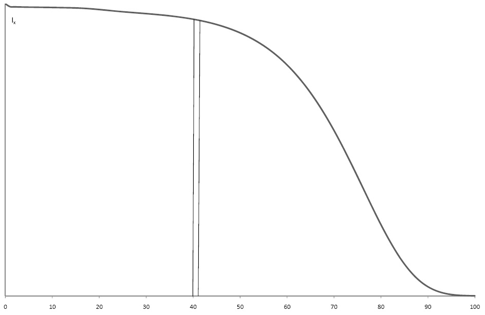
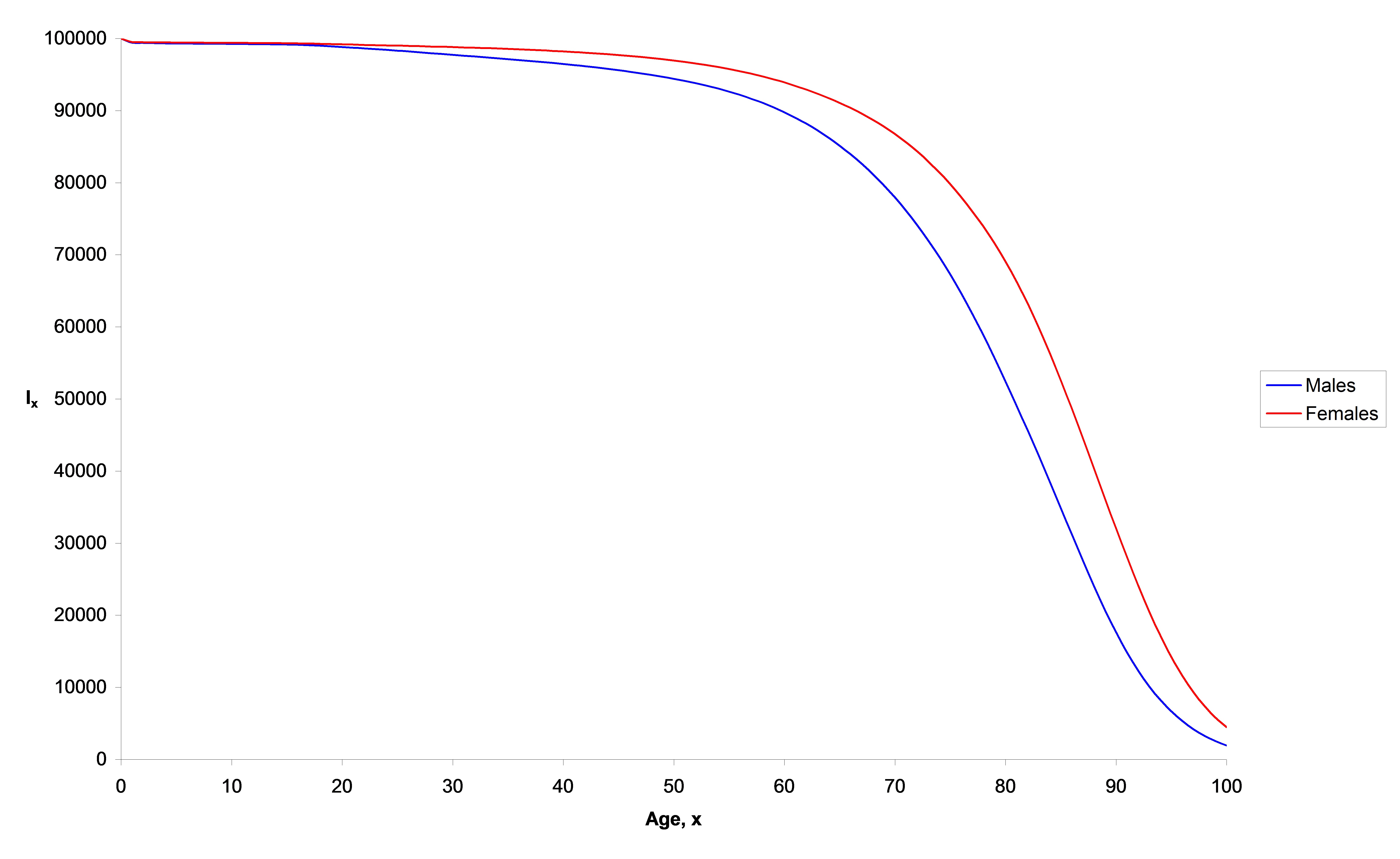
- the curve is
\(l_x\) - the area under the curve between 40 and 41 is
\(L_{40}\)
\(T_x\): Aggregate \(L_x\)
#
Define
$$T_x=\int_x^\infty l_y dy=\int_0^\infty l_{x+t} dt, \qquad x=0, 1, 2, \ldots.$$
Properties:
\(T_x=L_x+L_{x+1}+\ldots=\sum_{y=x}^\infty L_y\)\(T_x=L_x+T_{x+1}\)
It can be shown that
$$\overset{\circ }{e}_x=\int_0^\infty \ _tp_x ,dt. $$
which means that
$$\overset{\circ }{e}_x=\frac{T_x}{l_x}. $$
\(\overset{\circ }{e}_x\) represents the expected future life time of \((x)\).
Additionally,
$$T_x=l_x \overset{\circ }{e}_x$$
represents the expected total future life time of a group of \(l_x\) lives all aged \(x\).
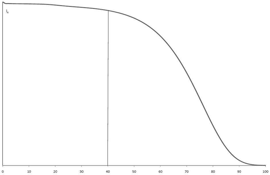
- the curve is
\(l_x\) - the area on the RHS of the vertical line at 40 is
\(T_{40}\)
Stationary populations #
Let us conduct the following thought experiment: Let us assume the table represents a stationary population. This means that the number entering the population each year is the same as the number leaving it:
- the number of births is equal to the number of deaths if immigrations and emigrations are not considered.
\((\Sigma d_x = l_0)\) - the population size is unchanged with time (zero growth rate);
- the size of a certain age group is unchanged with time;
- the mortality rate
\(q_x\)for each age remains the same from year to year; - we assume births are uniformly distributed throughout the year.
We can further interpret:
\(l_{x}\)is the number of people in the population who have their\(x\)-th birthday each year\(d_x\)is the number of deaths for each year between age\(x\)and\(x+1\). Note\(d_x\)does not change from one year to another.\(\sum_{x=0}^\infty d_x=l_0\)says that the number of deaths is the same as the number of births.\(L_x=l_x\int_0^1 \ _tp_xdt\)is the population size between ages\(x\)and\(x+1\)(aged\(x\)last birthday) at any time point.\(T_x=\sum_{y=x}^\infty T_y\)is the population size above age\(x\)at any time point.\(T_0=\sum_{y=0}T_y\)is the total population at any time during the stationary period.\(T_0-T_x\)is the population aged under age\(x\), aged\(0, 1, 2, \cdots x-1,\)last birthday.
Why does \(L_0\) represent the population aged \(0\) last birthday in a stationary population?
- Recall that
\(l_0\)is the number of births into a stationary population each year;\(l_x\)is the number of lives having their\(x\)-th birthday in each year.\begin{eqnarray*} L_0&=&\int_0^1 l_tdt=l_0\int_0^1 \ _tp_0dt=\lim_{n\to\infty} \sum_{k=0}^{n-1} \frac{l_0}{n} \ _{\frac{k}{n}}p_0\\ &\approx&\frac{l_0}{365}\left[\ _0p_0+\ _{\frac{1}{365}}p_0+\ _{\frac{2}{365}}p_0+\cdots+ \ _{\frac{k}{365}}p_0+\cdots+\ _{\frac{364}{365}}p_0\right]\,. \end{eqnarray*} - We assumed that births are uniformly distributed over the year, then
\(l_0/365\)is the number of births for each day over a year.
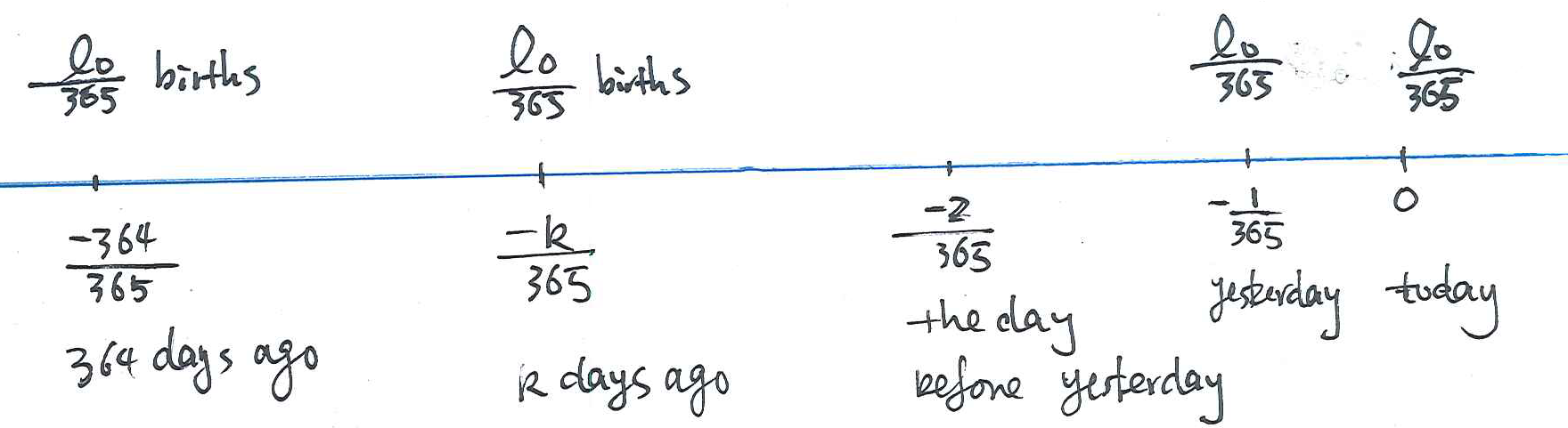
- the numbers of births today (aged 0 exactly today) is
$$\frac{l_0}{365}\ _0p_0=\frac{l_0}{365}$$ - the number of lives born yesterday surviving to today, aged 1 day or
\(1/365\)year at today, is$$\frac{l_0}{365} \ _{\frac{1}{365}}p_0$$ - Similarly,
$$\frac{l_0}{365} \ _{\frac{k}{365}}p_0$$is the number of lives born\(k\)days ago surviving to today, aged\(k\)days or\(k/365\)year at today. - Finally,
\(\frac{l_0}{365} \ _{\frac{364}{365}}p_0\)is the number of lives born\(364\)days ago surviving to today, aged\(364\)days or\(364/365\)year at today.
Wrapping up, $$ \textstyle L_0=\frac{l_0}{365}\ _0p_0+\frac{l_0}{365}\ _{\frac{1}{365}}p_0 +\cdots+ \frac{l_0}{365}\ _{\frac{k}{365}}p_0+\cdots+\frac{l_0}{365}\ _{\frac{364}{365}}p_0$$` is the numbers of lives aged under one year old.
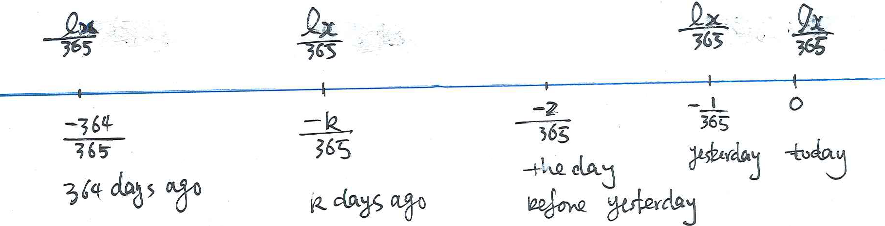
Now generalising, why does \(L_x\) represent the population aged \(x\) last birthday in a stationary population?
- We assumed that birthdays are uniformly distributed over the year, then
\(l_x/365\)is the number of lives having the\(x\)-th birthday for each day over a year.\begin{eqnarray*} L_x&=&\int_0^1 l_{x+t}dt=l_x\int_0^1 \ _tp_xdt=\lim_{n\to\infty} \sum_{k=0}^{n-1} \frac{l_x}{n} \ _{\frac{k}{n}}p_x\\ &\approx&\frac{l_x}{365}\ _0p_x+\frac{l_x}{365}\ _{\frac{1}{365}}p_x+\cdots+ \frac{l_x}{365}\ _{\frac{k}{365}}p_x+\cdots+\frac{l_x}{365}\ _{\frac{364}{365}}p_x\,. \end{eqnarray*}
Example 8 #
The following is an extract from a published life table.
\(x\) |
\(l_{x}\) |
\(d_{x}\) |
\(p_{x}\) |
\(\mu_x\) |
\(L_x\) |
\(T_x\) |
|---|---|---|---|---|---|---|
| 0 | 100,000 | 986 | 0.99014 | 0.01520 | 99,424 | 6,909,573 |
| 1 | 99,014 | 66 | 0.99933 | 0.00529 | 98,942 | 6,810,149 |
| 2 | 98,948 | 40 | 0.99960 | 0.00054 | 98,927 | 6,711,208 |
| 3 | 98,908 | 30 | 0.99970 | 0.00035 | 98,892 | 6,612,281 |
| 4 | 98,878 | 26 | 0.99974 | 0.00028 | 98,865 | 6,513,389 |
| 5 | 98,852 | 24 | 0.99976 | 0.00025 | 98,840 | 6,414,524 |
- Calculate the probability that a newborn life survives to age 5. Give your answer to 5 decimal places.
- Calculate the probability that of two lives aged 2, exactly one of them survives to age 5. Give your answer to 5 decimal places. You may assume that these two lives are independent with respect to mortality.
- Calculate
\(\overset{\circ} {e}_5=\text{E}[T(5)]\), the expected future life time of a life aged 5, from the life table above. Give your answer to 2 decimal places. - Estimate the probability that a baby aged exactly 1 will die in two days. Give your answer to 5 decimal places
Answers:
\(\ _5p_0=l_5/l_0=0.98852\)\({_3p}_2{_3q}_2+{_3q}_2{_3p}_2=2\times \frac{l_5}{l_2}\left(1-\frac{l_5}{l_2}\right)=0.00194\)\(\overset{\circ }{e}_5=E[T(5)]=T_5/l_5=64.89.\)- The estimated probability is
\(\mu_1\times (2/365)=0.00003.\)
Example 9 #
The population of a country experience the mortality of the life table in Example 8. The population of this country has reached a stationary condition with \(100,\!000\) births for each year during the stationary period. Calculate the following quantities to 2 decimal places:
- the crude birth rate (CBR) for this country,
- the crude death rate (CDR) for this country,
- the population size aged under 5.
Answers:
$$\text{CDR}=1,\!000\frac{\text{number of births}}{\text{population size}}=1,\!000\times\frac{l_0}{T_0}=1,\!000\times \frac{100,\!000}{6,\!909,\!573}=14.47$$- CBR=CDR, as the number of births is equal to the number of deaths in a stationary population.
\(T_0-T_5=495049.\)
Curtate future lifetime #
Expected Value of a Discrete Random Variable #
Suppose a random variable, \(X\), can take \(n\) values labelled \(x_{1},x_{2},...,x_{n}\).
The expected value of the random variable \(X\) (denoted \(E[X]\)) is
calculated using
$$E[X]=\sum_{i=1}^{n}x_{i}\Pr [X=x_{i}]. $$
Curtate future lifetime #
Recall: \(T(x)\) is the future lifetime of \((x)\).
We define a random variable
$$K(x)=\lfloor T(x) \rfloor$$
to be the number of whole years of future lifetime from age \(x\).
We call \(K(x)\) the curtate future lifetime at age \(x\).
For example:
- if (40) dies at age 75.6,
\(T(40)=35.6\), and\(K(40)=35\) - if (30) dies at age 82.3,
\(T(30)=52.3\), and\(K(30)=52\)
Pmf of \(K(x)\)
#
How do we find \(\Pr (K(x)=10)?\)
Answer: \(K(x)=10\) if \(10\leq T(x)<11.\)
Thus,
\begin{eqnarray*} \Pr [K(x)=10] &=&\Pr [10\leq T(x)<11] \\ && \\ &=& \frac{s(x+10)-s(x+11)}{s(x)} \\ && \\ &=& \ _{10}p_{x}-\ _{11}p_{x}. \end{eqnarray*}
Generalising:
$$\Pr [K(x)=k]=\ _{k}p_{x}-\ _{k+1}p_{x}$$
Curtate expectation of life #
The expected value of \(K(x)\) is called the curtate expectation of life at age \(x\), and is denoted \(e_{x}\). That is,
$$E[K(x)]=e_{x}.$$
The quantity \(\overset{\circ }{e}_x=E[T(x)]\) is called the complete expectation of life, and
$$\overset{\circ }{e}_x\approx e_{x}+\frac{1}{2}.$$
Using the pmf obtained earlier we have:
$$e_{x}=E[K(x)]=\sum_{k=0}^{\infty }\ k\times \Pr [K(x)=k]=\sum_{k=1}^{\infty }\ k\left(_{k}p_{x}-\ _{k+1}p_{x}\right)$$
Developing yields
\begin{eqnarray*} e_{x} &=& \sum_{k=1}^{\infty}\ k\left(_{k}p_{x}-\ _{k+1}p_{x}\right) \\ &=&\ _{1}p_{x}-\ _{2}p_{x}+2\left( \ _{2}p_{x}-\ _{3}p_{x}\right) \\ &&+3\left( \ _{3}p_{x}-\ _{4}p_{x}\right) +4\left( \ _{4}p_{x}-\ _{5}p_{x}\right) +\ldots \\ &=& \ _{1}p_{x}+\ _{2}p_{x}+\ _{3}p_{x}+\ _{4}p_{x}+\ldots \end{eqnarray*}
Thus, we get the important formula, $$e_{x}=\sum_{k=1}^{\infty }\ _{k}p_{x}\text{.} $$
Example 10 #
Consider the survival function
$$s(x)=\exp {-\lambda x} $$
where \(\lambda >0\).
Show that \(e_{x}\) is independent of \(x\).
Solutions:
We have $${}_{k}p_{x}=\frac{s(x+k)}{s(x)}=\frac{\exp \{-\lambda (x+k)\}}{\exp \{-\lambda x\}} = \exp\{-\lambda k \}$$
Thus
\begin{eqnarray*} e_{x} &=&\sum_{k=1}^{\infty }\ _{k}p_{x} \\ &=& \sum_{k=1}^{\infty }\exp \{-\lambda k\} \\ &=& \frac{\exp \{-\lambda \}}{1-\exp \{-\lambda \}} \end{eqnarray*}
which is independent of \(x\).
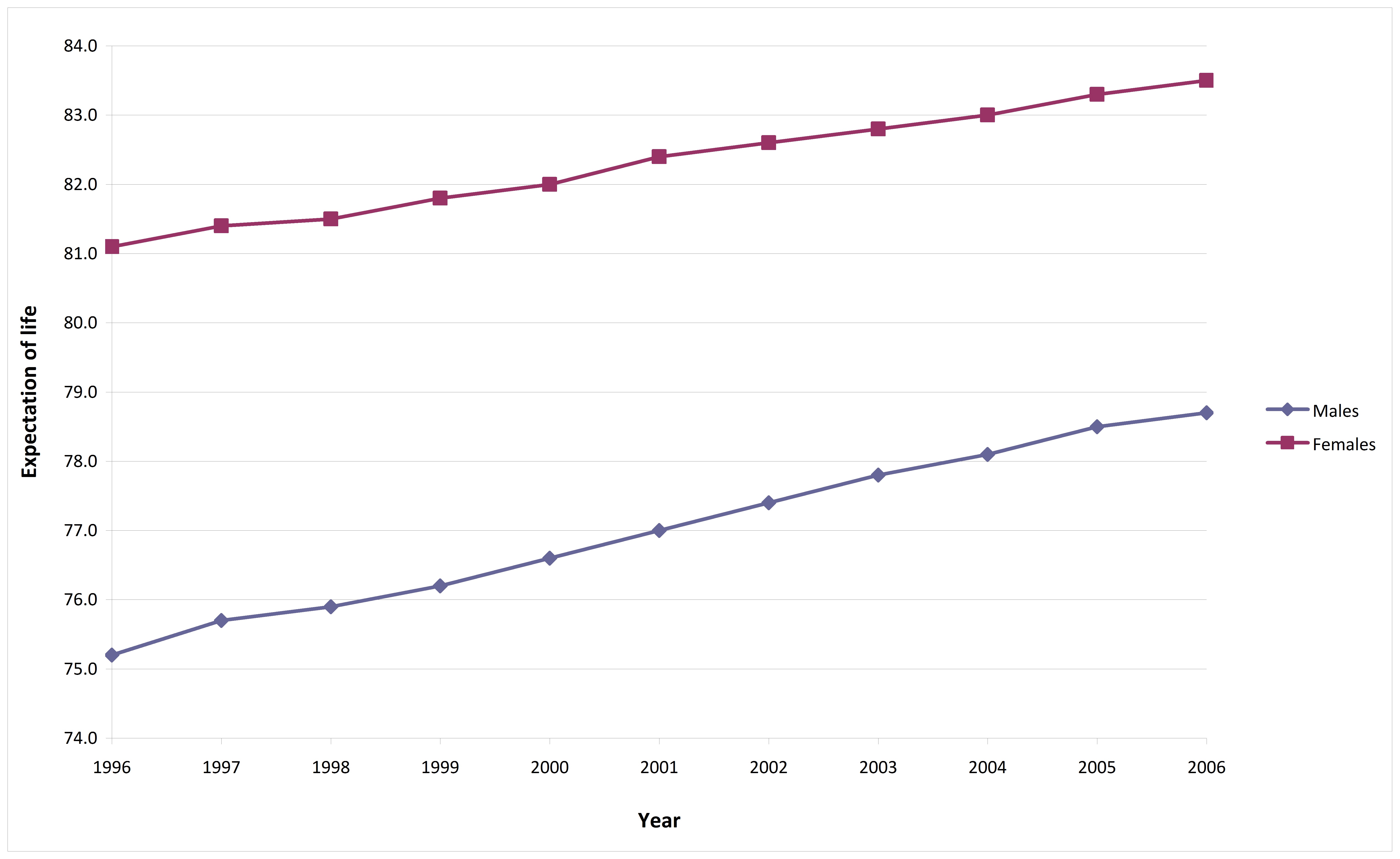
Expectation of life in Australia #
The plot shows expectation of life at birth in Australia. Source: ABS
Expectation of life around the World #
The table shows expectation of life from birth in 2005 for some countries.
| Country | Expectation of Male Life | Expectation of Female Life |
|---|---|---|
| Belgium | 75.44 | 81.94 |
| Canada | 78.55 | 83.54 |
| Kenya | 53.35 | 53.10 |
| Nicaragua | 68.27 | 72.49 |
| Pakistan | 62.04 | 64.01 |
| Singapore | 79.05 | 84.39 |
Source: US Census Bureau
These are life expectations calculated using a period table. They are often misinterpreted.
Period vs Cohort tables #
- Period tables describe mortality of a population in a given year (so different individuals of different age, all in the same calendar year). So there are potentially different period tables for different calendar years of death.
- Cohort tables look at the mortality of people born in the same calendar year – they track mortality of a given cohort. So there are potentially different cohort tables for different calendar years of birth.
Characteristics, causes and trends of mortality experience #
- Life tables are very important in traditional actuarial work.
- They are constructed from past experience, but may also include an allowance for ‘improving mortality’ – changes in mortality rates since the data were collected.
- Different tables are constructed based on different ‘exposed to risk.’ Calculations of quantities such as premiums are based on the assumption of a particular mortality experience, perhaps adjusted in some way – using the rate for a higher or lower age, or making a percentage loading on the tabulated rate.
- For example, there are tables based on annuitants’ data, which reflect the mortality experience of people who have purchased annuities. These people expect to have low mortality, otherwise they would not buy an annuity – they are ‘self selecting’ on this basis.
- Australian Life Tables are based on the whole Australian population, without any special features to affect their experience. We would expect the mortality rates to be higher than for annuitants.
- On the other hand, those who buy life insurance are insuring their lives and so are self-selecting on that basis – so we would expect, and we find, that their mortality rates are higher than for annuitants.
- So, choosing the appropriate table, and whether and how to adjust the rates is of primary importance in actuarial calculations.
In what follows, we illustrate some of the main features of human mortality in Australia.
Australian Life Tables 2000-02 #
This graph shows \(l_{x}\).
Australian Life Tables 2000–02 – Mortality Rates #
This graph shows \(q_{x}\) on a logarithmic scale.
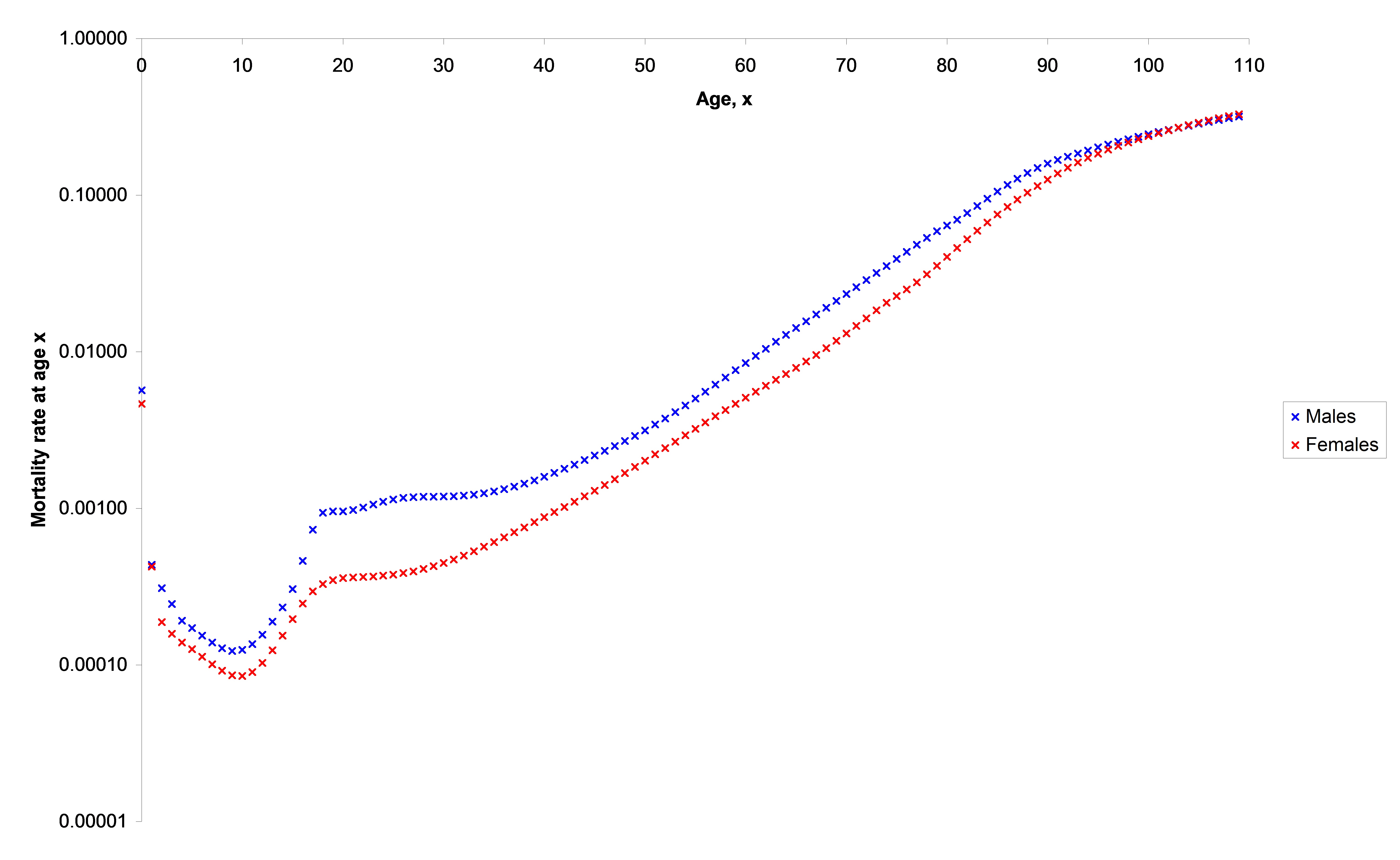
Australian Life Tables 2000–02 – Mortality Rates #
Some of the key features include:
- Life in the first years is risky.
- There is a ‘bump’ around the late twenties, where accidental death from risky behaviour becomes noticeable for males. This has tended to reduce for males, and increase for females.
- Mortality rates start to increase more steeply around ages 40-45.
Mathematical models of mortality #
Two theoretical models #
- Various ‘laws of mortality’ have been proposed over the years.
- Two old and famous ones are:
- Gompertz Law (1825):
$$\mu _{x}=Bc^{x},$$where\(B>0\),\(c>1\). This suggests that the force of mortality increases exponentially with age. - Makeham’s Law (1860):
$$\mu _{x}=A+Bc^{x},$$where\(A,B>0\),\(c>1\). Additionally, mortality is subject to a constant force,\(A\), that is independent of age – e.g. death by accidental causes.
- Gompertz Law (1825):
- How do these compare to mortality nowadays?
The force of mortality in Australia #
The plot shows \(\mu _{x}\) for males on a logarithmic scale – from
Australian Life Tables Males 2000-02.
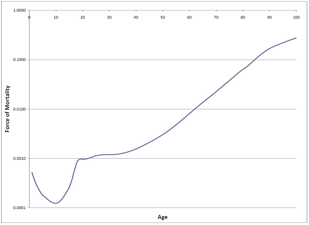
We observe that the force of mortality graph looks similar to a plot
of \(q_{x}\), namely
- decreasing at young ages,
- increasing in late teens/early twenties, and
- increasing as age increases.
This is typical in the developed world.
How does that compare with a formula like \(\mu _{x}=Bc^{x}\) which says
that \(\mu _{x}\) increases with \(x\)?
Gompertz law on a portion of Australian data #
The following plot shows Gompertz law fitted to Australian Life Tables Males
2000-02, for ages 50–100; \(q_{x}\) is plotted in red.
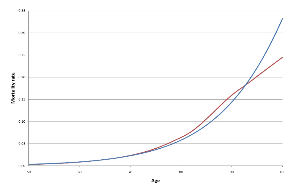
How was that fitted?
- In Australian Life Tables 2000–02 Females,
\(\mu _{50}=0.00193\)and\(\mu _{70}=0.01246.\) - We set
\begin{eqnarray*} \mu _{50} &=&0.00193=Bc^{50}, \\ \mu _{70} &=&0.01246=Bc^{70}. \end{eqnarray*} - Then
$$c^{20}=6.45596$$and so$$B=1.8224\times 10^{-5}.$$ - Hence an estimate of
\(\mu _{60}\)would become$$\mu _{60}=Bc^{60}=0.00490.$$(The published value is 0.00488.) - Estimates in the tail would be quite off.
Measures of fertility #
Definitions #
- Births are a natural source of increase for national populations. Another source of increase is immigration. Here we focus on births only.
- There are a number of summary statistics commonly used to describe features of fertility experience, such as
- General Fertility Rate (GFR)
- Age Specific Fertility Rate (ASFR$_x$)
- Total Fertility Rate (TFR)
- Gross Reproduction Rate (GRR)
- Net Reproduction Rate (NRR)
General Fertility Rate (GFR) #
$$\text{GFR}=1,!000\times \frac{\text{# of live births}}{\text{# of women aged } [15, 49]} $$ This is calculated as the number of live births per 1,000 women of reproductive age in a population.
The calculation is based on births in a fixed period of time, usually a calendar year.
In Australia, there were \(265,\!949\) live births in 2006. Thus, using the
corresponding population data, the GFR is
$$1,!000\times \frac{265,!949}{4,!918,!284}=54.07 $$
where we have taken women aged 15–49 to be of reproductive
age.
Comments on GFR #
- Crude Birth Rate (CBR)
$$\text{CBR}=1,!000\times \frac{\text{# of live births}}{\text{Population size }} $$
and hence we have
$$\text{GFR} > \text{CBR}.$$ - While GFR is better than CBR, a disadvantage of GFR is that it will be affected by the age distribution of women aged 15-49, which reduces its comparability.
In what follows we define the age specific fertility rates (ASFR) which are independent of the age distribution of the female population.
Age Specific Fertility Rate ( \(\text{ASFR}_x\) ) and Total Fertility Rate (TFR)
#
-
The Age Specific Fertility Rate (
\(\text{ASFR}_x\)) is defined as the number of live births per 1,000 women of a specific age or an age group in a (calendar) year: $$\text{ASFR}_x=1,!000\times \frac{\text{# of live births by women aged} [x, x+1)}{\text{# of women aged} [x, x+1)} $$\(ASFR_{x}\)is the the number of live births per 1,000 women aged\(x\). -
The Total Fertility Rate (TFR) is
$$\text{TFR}=\sum_{x=15}^{49}ASFR_{x}$$
- The ASFR can also be defined as fertility rates of women aged over an age group, 15-19, 20-24, 25-29, etc. For example,
$$\text{ASFR}_{[15, 19]}=1,\!000\times \frac{\text{\# of live births by women aged} [15, 19]}{\text{\# of women aged} [15, 19]}$$ - Thus, we could use the ASFR to compare, e.g., fertility rates of women aged 30–34 in Victoria and NSW without concerning ourselves with the population structure in these states.
Comparison of TFR with GFR #
Consider the following data in a given year:
| age | 15 | 16 | \(\cdots\) |
\(x\) |
\(\cdots\) |
49 |
|---|---|---|---|---|---|---|
| # of women | \(w_{15}\) |
\(w_{16}\) |
\(\cdots\) |
\(w_{x}\) |
\(\cdots\) |
\(w_{49}\) |
| # of live births | \(b_{15}\) |
\(b_{16}\) |
\(\cdots\) |
\(b_{x}\) |
\(\cdots\) |
\(b_{49}\) |
\begin{eqnarray*} \text{ASFR}_x&=&1,\!000\times \frac{b_x}{w_x},\qquad x=15, 16, \ldots, 49,\\ \text{TFR}&=&\sum_{x=15}^{49}1,\!000 \frac{b_x}{w_x}=\sum_{x=15}^{49} \text{ASFR}_x \end{eqnarray*}
Now, the GFR was calculated as
\begin{eqnarray*} \text{GFR}&=&1,\!000\frac{\sum_{x=15}^{49} b_x}{\sum_{x=15}^{49} w_x} \text{ which can be rewritten as}\\ &=&1,\!000\sum_{x=15}^{49}\frac{b_x}{\sum_{x=15}^{49} w_x} = 1,\!000\sum_{x=15}^{49}\frac{w_x}{\sum_{x=15}^{49} w_x}\frac{b_x}{w_x} =\sum_{x=15}^{49}\theta_x\, \text{ASFR}_x \end{eqnarray*}
Here
$$\theta_x=\frac{w_x}{\sum_{x=15}^{49} w_x} $$
is the percentage of women aged \(x\) last birthday to the total number of women at reproductive ages, with \(\sum_{x=15}^{49}\theta_x=1.\)
This is what changes from one population to another in the GFR, and which is somewhat standardised in the TFR (equal weights). In other words: If the proportion of women changes from one population to another, everything else being equal, this will impact the GFR but not the TFR.
Similarly, the age specific fertility rate over an age interval, say \([15, 19]\), is
\begin{eqnarray*} \text{ASFR}_{[15, 19]}&=&1000\frac{\sum_{x=15}^{19} b_x}{\sum_{x=15}^{19} w_x}=1000\sum_{x=15}^{19}\frac{b_x}{\sum_{x=15}^{19} w_x}\\ &=&1000\sum_{x=15}^{19}\frac{w_x}{\sum_{x=15}^{19} w_x}\frac{b_x}{w_x} =\sum_{x=15}^{19}\tau_x\, \text{ASFR}_x \end{eqnarray*}
where
$$\tau_x=\frac{w_x}{\sum_{x=15}^{19} w_x},\qquad x=15, 16, 17, 18, 19, $$ is the percentage of women aged \(x\) last birthday to the total number of women aged \([15, 19]\), with \(\sum_{x=15}^{19}\tau_x=1.\)
Summary #
\(\text{ASFR}_{[15, 19]}\)is the weighted average of\(\text{ASFR}_x\)over age interval\([15, 19]\).- GFR is the weighted average of
\(\text{ASFR}_x\)over the whole reproductive age interval\([15, 49]\). - TFR is the sum of
\(\text{ASFR}_x\)over all reproductive ages. - TFR is the number of the live births per 1000 women over their reproductive ages, assuming no mortality.
- To sustain population,
\(\text{TFR}/1000\ge 2.1\)
(roughly, but that depends on mortality etc…)- 2.1 is called the replacement level fertility.
- In Australia,
\(\text{TFR}/1000=1.88\)in 2013;\(\text{TFR}/1000=1.83\)in 2014;\(\text{TFR}/1000=1.81\)in 2015;\(\text{TFR}/1000=1.77\)in 2016;
Age Specific Fertility Rates in Australia #
The chart below shows ASFRs for Australia over the period 1999–2009.
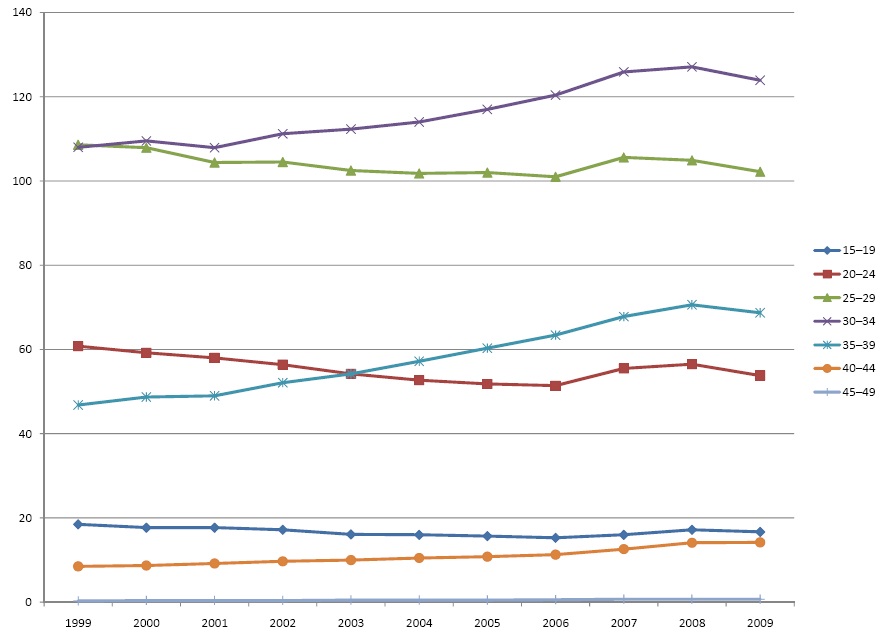
Observations:
- Fertility rates have fallen for women in their 20s
- Fertility rates have risen for women in their 30s
- There is a downward trend at ages 15–19 and an upward trend at 40–44, but these are small changes compared with other age groups.
- No real change at ages 45-49.
Gross Reproduction Rate (GRR) #
- Fertility rates tell us about how many babies are being born.
- Reproduction rates focus on the birth of female babies, because they are the only ones who will eventually be able to have babies themselves, later on. As the sex ratio at birth changes from one population to another (and also potentially across ages) then this makes a difference.
- Let
\(ASFR_{x}^{f}\)denote the ASFR$_x$ for female births. - Thus,
\(ASFR_{x}^{f}\)is defined as the number of live female births per 1,000 women at age\(x\)(per year). - The Gross Reproductive Rate (GRR) is then defined as $$GRR=\sum_{x=15}^{49}ASFR_{x}^{f} . $$
Comparison of TFR with GRR #
Remember
$$\text{TFR}=\sum_{x=15}^{49}ASFR_{x}$$
The sex ratio at birth is 1.05 (males vs females) on average, therefore we could estimate
$$ASFR_{x}^{f}=\frac{1}{2.05}ASFR_{x},\qquad\qquad x=15, 16, \ldots, 49. $$
and hence $$\text{GRR}=\frac{1}{2.05} \text{TFR}.$$
If we assume we need
$$\text{TFR}/1,\!000\ge 2.1$$
then this translates into (dividing by 2.05)
$$\text{GRR}/1,!000\ge 2.1/2.05=1.024. $$
Example 11 #
The following data from ABS relate to Australia in 2006. Estimate the GRR.
| Age Group | ASFR |
|---|---|
| 15–19 | 15.4 |
| 20–24 | 51.6 |
| 25–29 | 100.8 |
| 30–34 | 120.1 |
| 35–39 | 63.3 |
| 40–44 | 11.3 |
| 45–49 | 0.6 |
Answer:
- The rates are per 5 year age group. When data are presented like this it is
standard practice to assume that the given ASFR applies at each age in a
group.
- Thus, e.g., we assume
\(ASFR_{15}=ASFR_{16}=\ldots =ASFR_{19}=15.4.\)
- Thus, e.g., we assume
- The same assumption applies to each age group, so
\begin{eqnarray*} \sum_{x=15}^{49}ASFR_{x} &=&\sum_{x=15}^{19}ASFR_{x}+\sum_{x=20}^{24}ASFR_{x}+\ldots +\sum_{x=45}^{49}ASFR_{x} \\ &=&5(15.4+51.6+\ldots +0.6)=1,\!815.5=\text{TFR}. \end{eqnarray*} - Our data are not split by gender, so if we assume a sex ratio at
birth of 1.05, we get
$$GRR\approx \frac{1}{2.05}1,\!815.5=885.6$$per 1,000 women.
Note that several layers of approximation were used here:
- We used grouped ASFR to approximate the TFR:
$$\text{TFR}\approx 5 \times ( \text{ASFR}_{[15, 19]}+\text{ASFR}_{[20, 24]}+\cdots+\text{ASFR}_{[40, 44]}+\text{ASFR}_{[45, 49]} )$$ - We estimated the female ASFR using sex ratios at birth.
- We used a single sex ratio for all ages.
Net Reproduction Rate (NRR) #
- This is defined as the number of live female births surviving to the ages their mothers were at their births per 1,000 woman in an age group.
- It is a measure of the rate at which a woman of age
\(x\)is reproducing herself – with another woman who has survived to age\(x\)– so the probability of surviving to the age of the mother is taken into account. - Thus,
$$NRR=\sum^{49}_{x=15}ASFR^f_x \frac{l_{x+1/2}}{l_0}\approx\frac{1}{2.05}\sum^{49}_{x=15}ASFR_x \frac{l_{x+1/2}}{l_0}$$ - Note that we assume that women giving birth at age
\(x\)are on average age\(x+1/2\)(because\(x\)is “last birthday” in the table of\(l_x\)), and hence we use the probability of survival to age\(x+1/2\). - Frequently the age range is 5 years, or 10. If so, remember that the average age is half way through this range.
Example 12 #
Calculate the NRR from the following data.
| Age Group | ASFR | Survival Factor |
|---|---|---|
| 15–19 | 15.4 | 0.99279 |
| 20–24 | 51.6 | 0.99107 |
| 25–29 | 100.8 | 0.98921 |
| 30–34 | 120.1 | 0.98703 |
| 35–39 | 63.3 | 0.98410 |
| 40–44 | 11.3 | 0.97991 |
| 45–49 | 0.6 | 0.97377 |
Assume that the survival factor applies from birth to the age in the middle of each age group.
Answer:
\begin{eqnarray*} \text{NRR}&=&\frac{1}{2.05}\Bigg[\sum_{x=15}^{19} \text{ASFR}_x\frac{l_{x+1/2}}{l_0}+\sum_{x=20}^{24} \text{ASFR}_x\frac{l_{x+1/2}}{l_0}+\cdots\\ &&+\sum_{x=45}^{49} \text{ASFR}_x\frac{l_{x+1/2}}{l_0}\Bigg]\\ &=&\frac{1}{2.05}\Bigg[\sum_{x=15}^{19} 15.4 \frac{l_{x+1/2}}{l_0}+\sum_{x=20}^{24} 51.6 \frac{l_{x+1/2}}{l_0}+\cdots +\sum_{x=45}^{49} 0.6 \frac{l_{x+1/2}}{l_0}\Bigg]\\ &=&\frac{5}{2.05}\Bigg[\frac{15.4}{l_0}\sum_{x=15}^{19} \frac{l_{x+1/2}}{5}+\frac{5.16}{l_0}\sum_{x=20}^{24} \frac{l_{x+1/2}}{5}+\cdots +\frac{0.6}{l_0}\sum_{x=45}^{49} \frac{l_{x+1/2}}{5}\Bigg]\\ &=&\frac{5}{2.05}\left[15.4 \frac{l_{17.5}}{l_0}+51.6\frac{l_{22.5}}{l_0}+\ldots+0.6\frac{l_{47.5}}{l_0} \right] \end{eqnarray*}
| Age Group | ASFR | Survival Factor | |
|---|---|---|---|
| (1) | (2) | (3) | (2) \(\times\) (3) |
| 15–19 | 15.4 | 0.99279 | 15.2889 |
| 20–24 | 51.6 | 0.99107 | 51.1392 |
| 25–29 | 100.8 | 0.98921 | 99.7119 |
| 30–34 | 120.1 | 0.98703 | 118.5417 |
| 35–39 | 63.3 | 0.98410 | 62.2932 |
| 40–44 | 11.3 | 0.97991 | 11.0730 |
| 45–49 | 0.6 | 0.97377 | 0.5843 |
Finally $$\text{NRR}=\frac{5}{2.05}\left( 15.2889+\ldots +0.5843\right) =874.7 $$ per 1,000 women.
Factors affecting fertility #
- Standards of nutrition, sanitation, and health more broadly mainly have an impact on child survival, but they do have some impact on the success of pregnancies (and the wish of parents to have children) as well.
- Then how many babies to have is mostly a matter of choice, and population circumstances have an impact on those choices:
- In general, increased prosperity leads to lower fertility rates.
- Individuals delay parenthood, and limit the number of children.
- Philosophical and religious convictions may have an impact, too.
- Some countries may decide to implement strict birth policies (e.g. China).
- Importantly, developing countries may have high fertility rates, but low reproduction rates, due to poor health. These highlight how different both types of indicators are.
Trends in fertility rates, and consequences #
- Trends in fertility rates for developing countries are typically as follows:
- Women are having fewer children over their reproductive lifetime.
- Women are choosing to have their first child later in life.
- Complete family size is falling.
- A consequence is an increase in generation gap, whereby parents are typically 30-40 years older than their children (as opposed to 20-30 years older).
- This, coupled with reduced mortality at all ages, leads to an ageing of the population, which has serious consequences.
- Recall the increasing age dependency ratio.
- Elderly people may not have large families available to care for them (they had no children, or they moved overseas), and there are less active people to fund their care (at society level).
Population projections #
- A population projection gives a profile of a population in the future, based on current (and past) data, and our view as to how the population will change over time.
- There are many reasons why we might be interested in knowing what a population will look like in the future. For example, to estimate the cost of providing a particular service (education, health care, social security payments, etc) to a particular group in the population.
- There are a number of different models and methods commonly used to estimate population size based on different types of growth.
Polynomial model #
Let \(P_{t}\) be the size of the population at time \(t.\) Then
$$P_{t}=P_{0}+\sum_{i=1}^{n}a_{i}t^{i}$$
for constants \(a_{1}\), \(a_{2}, \ldots,a_{n}\) and initial population \(P_0\).
As a special case, the linear model is
$$P_{t}=P_{0}+at=P_0(1+r t)\text{,} $$
where \(r=a/P_0\) is called a *simple* annual growth rate.
Geometric population growth #
This method assumes a compound rate of growth \(r\) per unit
time so that
$$P_{t}=P_{0}(1+r)^{t}$$
For example, we may use the information from past years and extrapolate to the future.
This method has the advantage that it is very simple to apply.
It has the disadvantage that it is very simplistic!
Example 13 #
A country’s population in 1990 was 12 million. In 2000 it was 14 million.
Assuming geometric population growth, project the country’s population in 2015.
Answer:
- We have
$$P_{2000}=(1+r)^{10}P_{1990} $$
giving
\((1+r)^{10}=\frac{7}{6}\). - Then
\begin{eqnarray*} P_{2015} &=&(1+r)^{15}P_{2000} = \left( 7/6\right) ^{1.5}\times 14\times 10^{6} \\ && \\ &=& 17.642\times 10^{6}. \end{eqnarray*}
Logistic model #
Populating growth under the logistic model is represented as
$$P_{t}=\frac{1}{A+Be^{-rt}}. $$
Thus, at \(t=0\)
$$P_{0}=\frac{1}{A+B}, $$
and there is a limiting population size as \(t \to \infty\),
$$\lim_{t\rightarrow \infty }P_{t}=\frac{1}{A}. $$
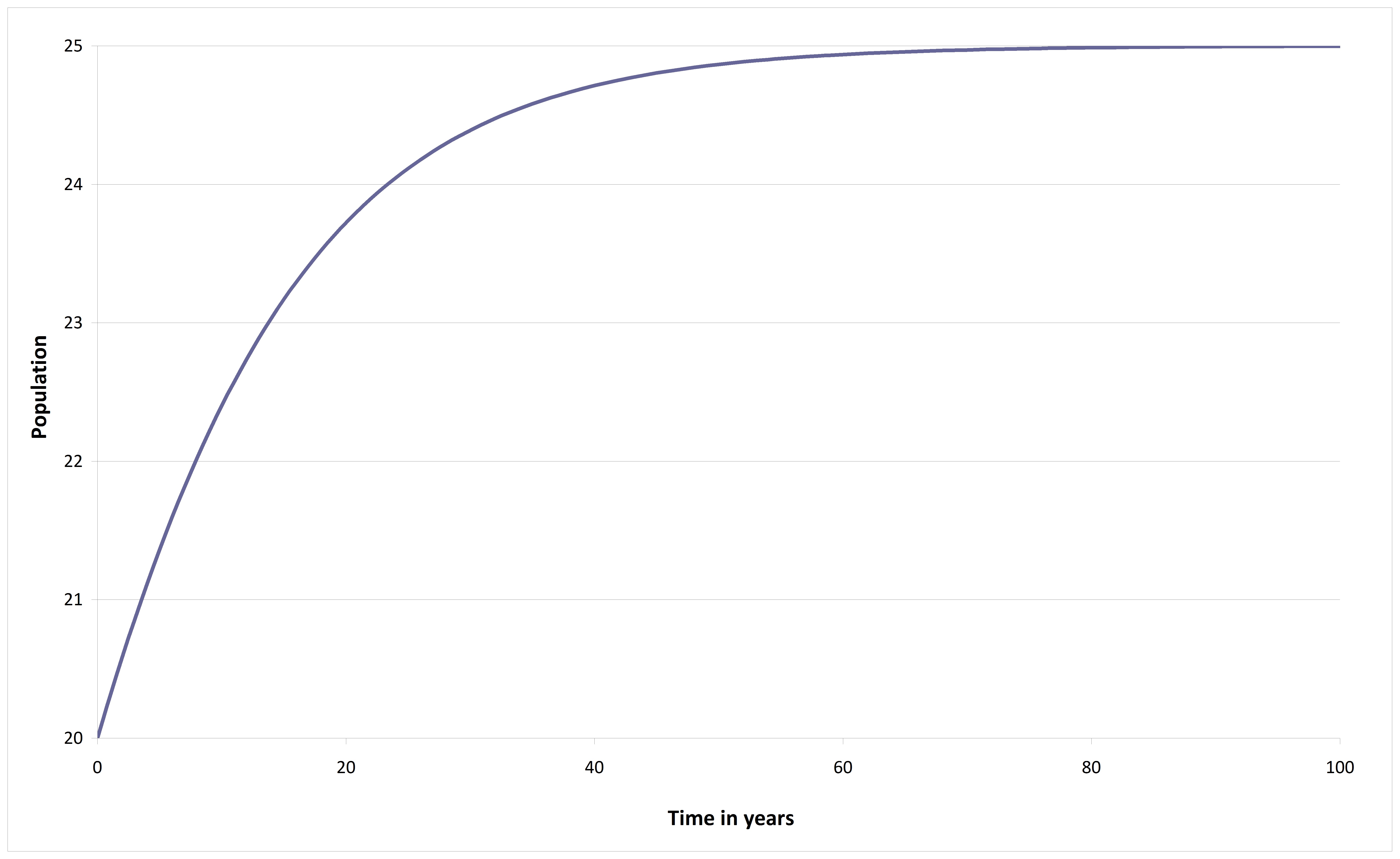
Example 14 #
The population of a certain country is currently 20 million.
The population is estimated to grow by 1.5% over the next year.
Assume that the population will grow to a limiting value of 25 million.
Estimate the population size in 50 years’ time under a logistic model
of population growth
$$P_{t}=\frac{1}{A+Be^{-rt}}.$$
Answer:
- We know `$$\lim_{t\rightarrow \infty }P_{t}=\frac{1}{A}=25\times 10^{6}\Rightarrow A=4\times 10^{-8}. $$
- Also, `$$P_{0}=\frac{1}{A+B}=20\times 10^{6}\Rightarrow A+B=5\times 10^{-8}\Rightarrow B=10^{-8}. $$
- Lastly, we know that
$$\frac{P_{1}}{P_{0}}=1.015=\frac{A+B}{A+Be^{-r}} $$
giving
\(r=0.076765\). - Thus, $$P_{50}=\frac{10^{8}}{4+\exp {-50r}}=24.87\times 10^{6}\text{.} $$
The population here grows as in the graph below.
Component method #
- Finally, there is the component method. This is detailed and models the ‘components’ which contribute to growth or decline of the population.
- Simply put,
$$P_{t}=P_{0}+[births-deaths+immigration-emigration]\quad (\text{from 0 to }t))$$The Australian Bureau of Statistics (ABS) website has apopulation clockshowing estimates of how Australia’s population is projected into the future. It uses such a component model. - This method enables assumptions about the mortality, fertility, immigration and emigration rates in as detailed a way as we wish.
- It also enables us to investigate the effects of different rates/assumptions have on future population growth and distributions (“what if” analysis), which is crucial for decision making.
References #
Here is the correspondance of sections with the book Atkinson and Dickson (2011):
- Section 1: 3.3.1
- Section 2: 3.3.2
- Section 3: 3.3.3
- Section 4: 3.3.4
- Section 5: 3.4
- Section 6: 3.5
Atkinson, M. E., and David C. M. Dickson. 2011. An Introduction to Actuarial Studies. 2nd ed. Edward Elgar.