Loans #
Introduction #
-
We now turn our attention to applying our knowledge of compound interest and annuities to analysing loans.
-
Suppose you wish to borrow an amount of money, say $100,000, from a bank. This amount, lent by the bank, is called the principal.
-
Of course, the bank will charge you interest on the balance of your loan.
The interest charged by the bank is generally quoted as a nominal (compound) interest rate.
For instance, it could be charged at 12% per annum, convertible monthly, i.e., \(i^{(12)}=12\%\).
Main components #
The main components of a loan are:
- principal
\(P\): the amount of money that is borrowed/lent - interest rate
\(i\), usually an\(i^{(m)}\)p.a. - repayments
\(X\)(which usually include an interest component, and a reimbursement component), usually paid every 1/$m$ years - maturity
\(T\)years - number of payments
\(n\), usually\(T\cdot m\). Typically, one has $$ P= X a_{\angl{T}\ i}$$ for annual repayments\(X\)in arrears or$$P = (mX) a_{\angl{T}\ i^{(m)}}^{(m)} = X a_{\angl{m\cdot T}\ i^{(m)}/m}$$for\(1/m\)-thly repayments\(X\)in arrears.
For instance, a 30 year housing loan at interest \(i^{(12)}\) becomes
$$P = X a_{\angl{360}\ i^{(12)}/12}$$
If \(P=100,\!000\), and \(i^{(12)}=12\%\) then \(X=1,\!028.61\).
Example 1 #
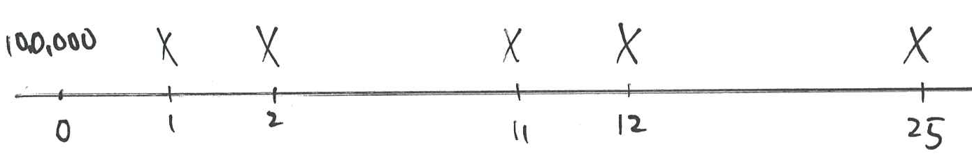
- Consider a $100,000 loan repayable by 25 equal annual instalments,
\(i=8\%\), per annum effective.- Let the instalment be
\(X\).
Calculate \(X\).
Solution: We have
$$100,!000=Xa_{\angl{25}} $$
at \(i=8\%\), giving
\begin{eqnarray*} X &=& 100,\!000 / a_{\angl{25}} \\ && \\ &=& 100,\!000\frac{0.08}{1-1.08^{-25}} \\ && \\ &=& \$9,\!367.88. \end{eqnarray*}
Loan repayment schedule #
A loan repayment schedule is a table which sets out the amount of the loan outstanding, the instalments paid, the interest charged and the capital repaid under a loan throughout its duration.
We define the following terms:
\(L_{t}\)= principal (or loan) outstanding at time\(t\)after the instalment then due has been paid.\(X\)= instalment.\(i\)= effective rate of interest in time period\(t\)to\(t+1\).\(C_{t}\)= capital repaid in instalment number\(t\).\(I_{t}\)= interest component of instalment number\(t\).
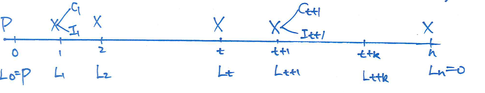
The following relationships hold between the above variables:
\begin{eqnarray*} I_{t+1} &=&L_{t}\times i, \\ \\ C_{t+1} &=& X-I_{t+1}=X-L_{t}\times i, \\ \\ L_{t+1} &=& L_{t}-C_{t+1}=L_{t}(1+i)-X \end{eqnarray*}
Example 2 #
Consider a loan for $200,000 with a term of three years. Interest is charged at 10% per annum effective and instalments are paid annually in arrears for three years.
- Calculate the annual instalment
\(X\). - Complete a loan repayment schedule for this loan, showing the loan outstanding at times 0,1,2 and 3 years as well as the repayments, interest charged and capital repaid at times 1, 2 and 3 years.
Solution:
- We set up the equation of value:
$$200,\!000=Xa_{\angl{3}}=X\ \frac{1-1.1^{-3}}{0.1},$$giving $X=$80,!422.96$. - The loan repayment schedule is given below:
Time, \(t\) (years) |
Payment | Interest due |
Principal repaid |
Outstanding balance |
|---|---|---|---|---|
| 0 | - | - | - | 200,000.00 |
| 1 | 80,422.96 | 20,000.00 | 60,422.96 | 139,577.04 |
| 2 | 80,422.96 | 13,957.70 | 66,465.26 | 73,111.78 |
| 3 | 80,422.96 | 7,311.18 | 73,111.78 | 0.00 |
Outstanding loan calculations #
There are three formulae for \(L_t, t=1, 2, \ldots, n\):
- Recursive formula:
$$L_{t+1}=L_t(1+i)-X, $$
with starting value is
\(L_0=P\). - Prospective formula: $$L_t=Xa_{\angl{n-t}},. $$
- Retrospective formula: $$L_t=P(1+i)^t-Xs_{\angl{t}} $$
Example 3 #
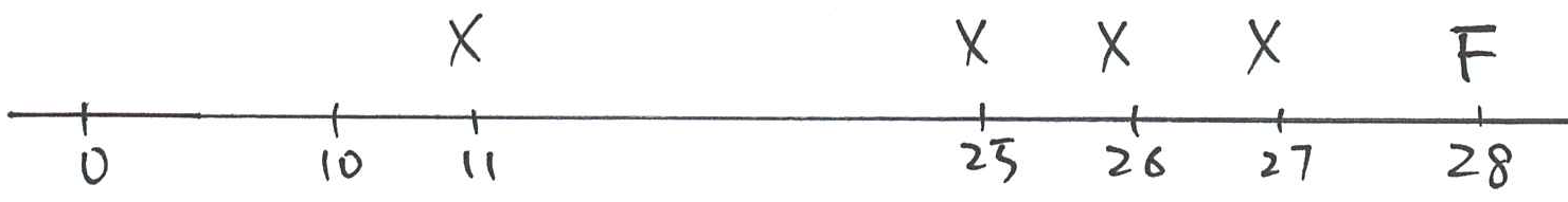
Consider again the loan in Example 2. How would you calculate the amount that the person who originally borrowed the $100,000 still owes the bank after 11 years?
After 11 years,
- 11 payments have been made under the loan,
- there are 14 payments (each equal to $9,367.88) remaining that still need to be paid.
Note that when we calculate the loan outstanding at the time of an instalment we assume that the instalment payable on the date when the outstanding loan is being calculated has already been paid.
Hence in the example given above, the loan outstanding after 11 years is (using the prospective formula) $$9,!367.88a_{\angl{14}}=9,!367.88\frac{1-1.08^{-14}}{0.08}=$77,!231.02.$$
Equivalence of prospective and restrospective formulas #
Here we derive the prospective and restrospective formulas from the recursive one, and show that these are all indeed equivalent.
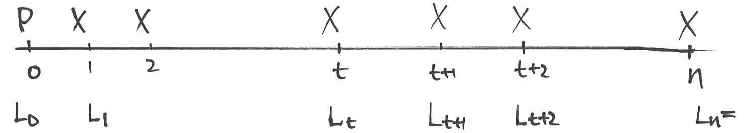
- We consider a loan of
\(P\)with a repayment period of\(n\)time periods. - Define
\(X\)to be the amount of the instalment paid at the end of each time period. - Define
\(L_{t}\)to be the amount of the loan outstanding after\(t\)time periods. Note that, of course,$$L_0= P,\quad\text{and }L_n=0.$$
Clearly, we have
\begin{eqnarray*} L_{t+1}&=&L_{t}(1+i)-X \\ L_{t+2} &=&L_{t+1}(1+i)-X \\ &=& L_{t}(1+i)^{2}-X(1+i)-X = L_{t}(1+i)^{2}-Xs_{\angl{2}}. \end{eqnarray*}
Similarly,
\begin{eqnarray*} L_{t+3} &=&L_{t+2}(1+i)-X \\ &=& L_{t}(1+i)^{3}-X(1+i)^{2}-X(1+i)-X \\ &=& L_{t}(1+i)^{3}-Xs_{\angl{3}}. \end{eqnarray*}
In general,
\begin{eqnarray} L_{t+k}=L_t\,(1+i)^{k}-X\,s_{\angl{k}},\quad t+k\le n. \label{A} \end{eqnarray}
Also noticing the emerging pattern, we have
$$L_{n}=L_{t}(1+i)^{n-t}-Xs_{\angl{n-t}} $$
or, equivalently, as \(L_{n}=0\),
$$Xs_{\angl{n-t}}=L_{t}(1+i)^{n-t}, $$
so that
$$L_{t}=Xs_{\angl{n-t}}(1+i)^{-(n-t)}=Xa_{\angl{n-t}}. $$
In particular,
$$L_{0}=Xa_{\angl{n}}. $$
Additional examples #
Example 4 #
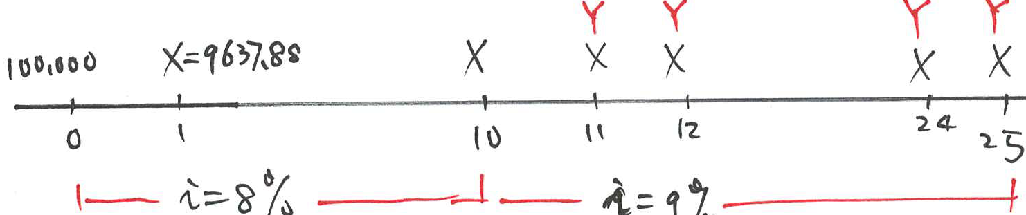
- A loan of $100,000 is repayable by equal annual instalments over 25 years at 8% per annum effective.
- The annual repayment required is $9,367.88 (from Example 1).
- Suppose that immediately after the 10th instalment is paid, the annual effective interest rate increases to 9%.
- Calculate the revised instalment so that the loan will still be repaid exactly 25 years after the funds were originally lent.
Solution:
- The strategy is to find the loan outstanding at the time when the interest rate changes and then use this loan outstanding as the amount owing that needs to be paid within 15 years.
- After 10 years, the loan outstanding is
$$9,\!367.88 a_{\angl{15}\ 8\% } = 9,\!367.88 \frac{ 1 - 1.08^{-15} }{0.08} = 80,\!184.15$$ - Now, if the annual effective rate of interest is 9%, we let the new
repayment be
\(Y\)and calculate:$$80,\!184.15=Ya_{\angl{15}\ 9\% }$$at 9%, so that$$Y=80,\!184.15\frac{0.09}{1-1.09^{-15}}=9,\!947.56$$
Example 5 #
- Again we consider our loan for $100,000 where after ten years the annual effective interest rate charged increases to 9% per annum effective.
- Suppose that the borrower refuses to pay the higher instalment but instead wishes to increase the term of the loan.
- Calculate the revised term of the loan.
- Suppose that the borrower pays instalments of $9,367.88 followed by a final reduced instalment in order to repay the loan. Calculate the amount of the final reduced instalment.
Solution:
- From Example 4, we know that after ten years the loan outstanding is
$80,184.15. This needs to be repaid using instalments of $9,367.88. We
therefore get
$$80,!184.15=9,!367.88\frac{1-1.09^{-n}}{0.09} $$
giving
$$1.09^{-n}=1-0.09\frac{80,\!184.15}{9,\!367.88}.$$Taking the\(log\)of each side we get\(n=17.1\).
Therefore we need 17 full repayments plus one final smaller repayment.
- Let the amount of the final instalment be
\(F\). We have $$80,!184.15=9,!367.88a_{\angl{17}}+Fv^{18} $$ or$$80,\!184.15=9,\!367.88\frac{1-1.09^{-17}}{0.09}+\frac{F}{1.09^{18}},$$giving\(F=700.19.\)
Example 6 #
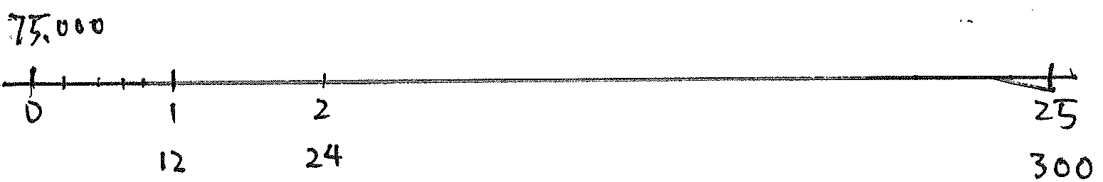
A loan of $75,000 is repaid by equal monthly instalments over 25 years with interest charged at 9% per annum convertible monthly.
- Calculate the monthly repayment amount
\(X\). - How much capital is repaid in the second year?
- How much interest is paid in the second year?
Solution:
- The amount of each instalment,
\(X\), is\begin{eqnarray*} X &=&\frac{75,\!000}{a_{\angl{300}}}\quad \text{at }i=0.0075 \\ &=&\frac{75,\!000\times 0.0075}{1-1.0075^{-300}} =\$629.40. \end{eqnarray*}
- To find the amount of the loan repaid (the capital repaid) in the second year, we need to calculate the difference between the loan outstanding at the start of the second year and the end of the second year.
Using\(L_{t}\)to denote the loan outstanding after\(t\)months, at\(i=0.0075\)we have: $$L_{12} =X,a_{\angl{288}} = 629.40 \frac{1-1.0075^{-288}}{0.0075} = $74,!163.28.$$ Similarly, we have\begin{eqnarray*} L_{24} &=&X\,a_{\angl{276}} \\ &=&629.40 \frac{1-1.0075^{-276}}{0.0075} \\ &=& \$73,\!248.06. \end{eqnarray*}Hence the capital repaid is $$74,!163.28-73,!248.06=$915.22.$$
- During the second year we know that 12 instalments are paid.
The total instalments paid in the second year are $$12\times X=12\times 629.40=$7,!552.80.$$ Therefore interest paid in the second year is $$7,!552.80-915.22=$6,!637.58.$$
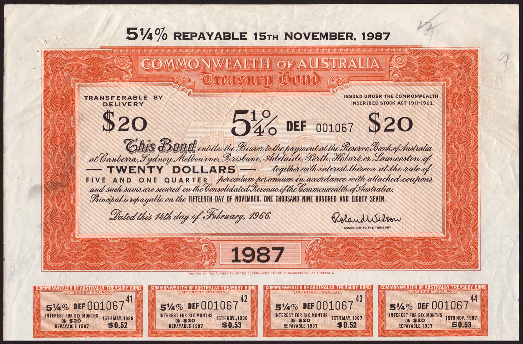
Bonds #
Introduction #
- Bonds are very large securitised loans, generally interest only until maturity
- Borrowers can be the government (e.g. T-Notes) or companies
- Because of the securitisation, some features are standardised:
- The loan is “cut” in small chunks (e.g. $10,000)
- The actual interest payments are fixed and don’t change over the life of the bond
- The principal, or face value is reimbursed at maturity
- Bonds are securities that can be traded. Because everything is set (“printed”) their price will depend on how much interest/yield the market wants to obtain from this borrower:
- the higher the risk, the higher the expected yield
- the higher the inflation, the higher the expected yield
We will then need to learn how to calculate a price from a yield, and a yield from a price
(the latter is a lot more complicated than the former)
Prices and Yield to Maturity (YTM) #
- Three possible cases for the price
\(P\):- If
\(P=F,\)the bond is sold at par; - if
\(P<F,\)the bond is sold at a discount; - if
\(P>F,\)the bond is sold at a premium.
- If
- The “Yield to Maturity” (YTM) goes hand in hand with the price.
It is the interest rate that makes the present value of all remaining cash flows equal to the price
Some typical securities #
Review of treasury notes (T-Notes) #
- Short term government debt security.
- Terms are generally less than one year.
- T-notes are sold at a discount to the face value.
- The discount amount is calculated using simple interest rate
\(r\)or simple discount rate\(d\).
Fixed coupon treasury bonds #
- A bond is a type of financial instrument issued by an organisation that wishes to borrow money.
- A treasury bond (often called a T-bond) is a financial instrument issued by the government.
- A T-bond is a medium to long-term government security.
- A T-bond has a pre-specified face value (par value, nominal value), say
\(F\), at the maturity date\(T\). - A T-bond is sold to a buyer at time zero at a price
\(P\). - The government makes fixed interest payments of amount
\(C\)(coupons, dividends) semi-annually.
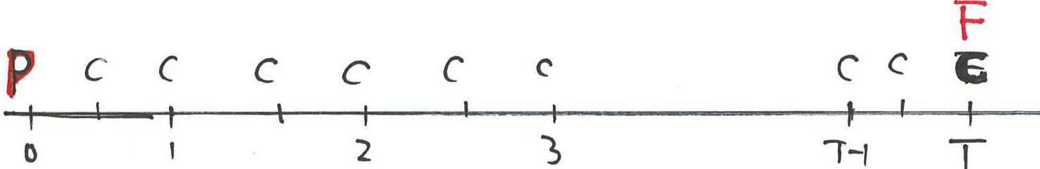
- The coupon rate is
\(2C/F\)
Example 7 #
- Let’s say that today’s date is the 10th October 2010.
- Suppose that the government wishes to borrow $100 today and that they will repay the $100 in five years’ time – that is, the government will repay the loan on the 10th October 2015.
- We say that the government issues a T-bond with face value (par value, nominal value) of $100.
- The lender or buyer of the T-bond will receive coupons from the government during the 5-year time.
- Suppose that the coupons are paid half-yearly with amount of $3.75 at the end of each half year until the maturity date (10th October 2015).

- The coupon rate is the annual coupon amount/face value. Here the coupon rate=7.5% per annum.
- Let
\(j^{(2)}\)be the yield per annum convertible half-yearly. Then we have\begin{eqnarray*} 100&=&3.75\,a_{\angl{10}}+100v^{10}\\ &=&3.75\frac{1-(1+j^{(2)}/2)^{-10}}{j^{(2)}/2}+100\left(1+j^{(2)}/2\right)^{-10}\,. \end{eqnarray*}This gives $$100 \left[1-\left(1+j^{(2)}/2\right)^{-10}\right]=\frac{7.5}{j^{(2)}}\left[1-\left(1+j^{(2)}/2\right)^{-10}\right], $$ if and only if\(j^{(2)}=7.5\%.\)
Remarks:
- If the purchasing price is equal to the face value, then the YTM is equal to the coupon rate.
- Hence annual interest payable will be $7.50 in our example. The semi-annual coupon will be $3.75.
Example 8 #
Following the information from previous page.
- You lend the government $100 today. They give you the $100 face value T-bond.
- Suppose now it is 10th October 2011 and you have just received your coupon of $3.75. You decide to sell the bond at this time.
- Let
\(P\)be the price that the buyer want to pay such that the yield on bonds is\(j^{(2)}=7.2\%\)per annum convertible half-yearly (from 10th October 2011 to 10th October 2015.
Calculate \(P\).
It is said that you are selling the bond ex-interest.
When you sell the bond you are giving the buyer the right to receive future payments, including
- Coupon payments of $3.75 payable on 10 April 2012, 10 October 2012,, 10 October 2015;
- face value of $100 from the government on 10 October 2015.
The bond price \(P\) is the PV of all these future payments at the date of sale of the bond.
We therefore calculate the price, \(P\), using
\begin{eqnarray*} P &=&3.75a_{\angl{8}}+100v^{8} \\ &=& 3.75\frac{1-1.036^{-8}}{0.036}+100(1.036^{-8}) \\ &=& 101.03. \end{eqnarray*}
Determining the YTM from a price #
The yield on a bond: #
- Suppose the above bond was to be sold on 10th October 2011, as in Example 8, however, the price of the bond on that day is $101.50.
- Let
\(j^{(2)}\)is the (nominal) yield per annum convertible half-yearly. - Then
\(j=j^{(2)}/2\)is the yield per half year implied by this bond. How would you calculate\(j\)?
Looking at the Solution to Example 8, it should be clear that we can set
up the following equation:
$$101.50=3.75a_{\angl{8}}+100v^{8} $$
evaluated at rate \(j\) per half year.
Our task is to calculate \(j\). Looking at the above equation, we can
write
$$101.50=3.75\frac{1-(1+j)^{-8}}{j}+100(1+j)^{-8} $$
or, equivalently, we write the above equation as
$$P(j)=3.75\frac{1-(1+j)^{-8}}{j}+100(1+j)^{-8}-101.50=0. $$
The above equation is non-linear in \(j\) and cannot be readily solved for \(j\). We therefore adopt the following approach to solving the above equation – the following is a method that you should know for calculating bond yields:
- Estimate the solution to the bond price equation using general reasoning.
- Find two estimated values of
\(j\), say,\(j_1\)and\(j_2\), such that\(P(j_1)>0\)and\(P(j_2)<0\). - Use linear interpolation to refine your estimate of
\(j\).
Estimation - Step 1 #
Estimate \(j\) using
$$j=\frac{3.75}{101.5}+\frac{(100-101.5)/8}{101.5}=0.0351.$$
There are two contributions to \(j\) – the coupon payments (3.75) and the capital gain (a loss of 1.5 here) at the end of the term, which both need to be compared with the initial price 101.5.
Estimation - Step 2 #
Calculate both
\begin{eqnarray*} P(0.035) &=&3.75\frac{1-(1.035)^{-8}}{0.035}+100(1.035)^{-8}-101.50 \\ &=&0.2185 \end{eqnarray*}
and
\begin{eqnarray*} P(0.036) &=&3.75\frac{1-(1.036)^{-8}}{0.036}+100(1.036)^{-8}-101.50 \\ &=&-0.4732. \end{eqnarray*}
Hence the true solution, the true yield per half year, \(j\), lies
between 3.5% and 3.6%.
Estimation - Step 3 #
We assume that the function \(P(j)\) is linear between \(j=0.035\) and \(j=0.036\). The plot below shows \(P(j)\) – it is not linear, but assuming linearity is reasonable for small interest spreads.
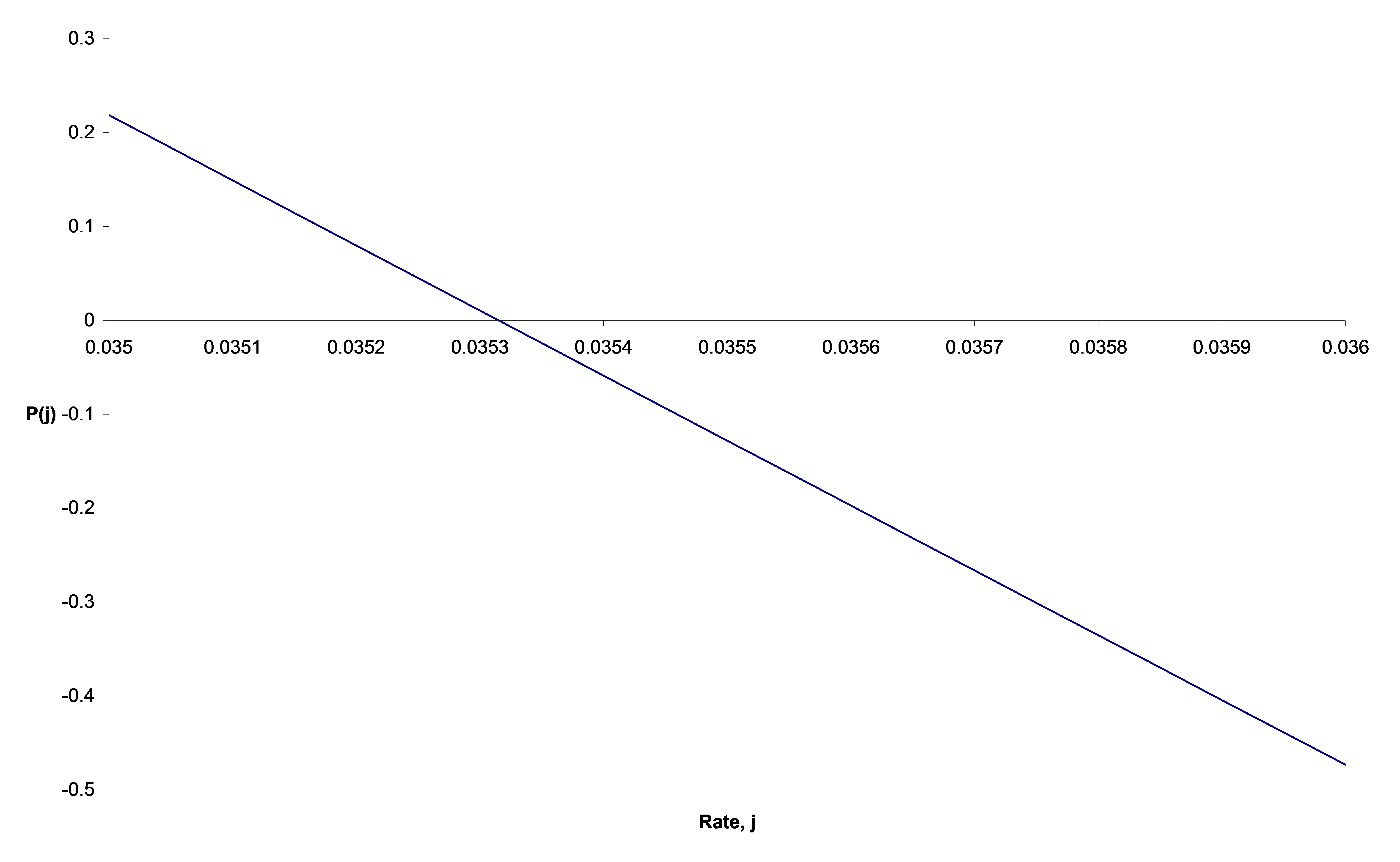
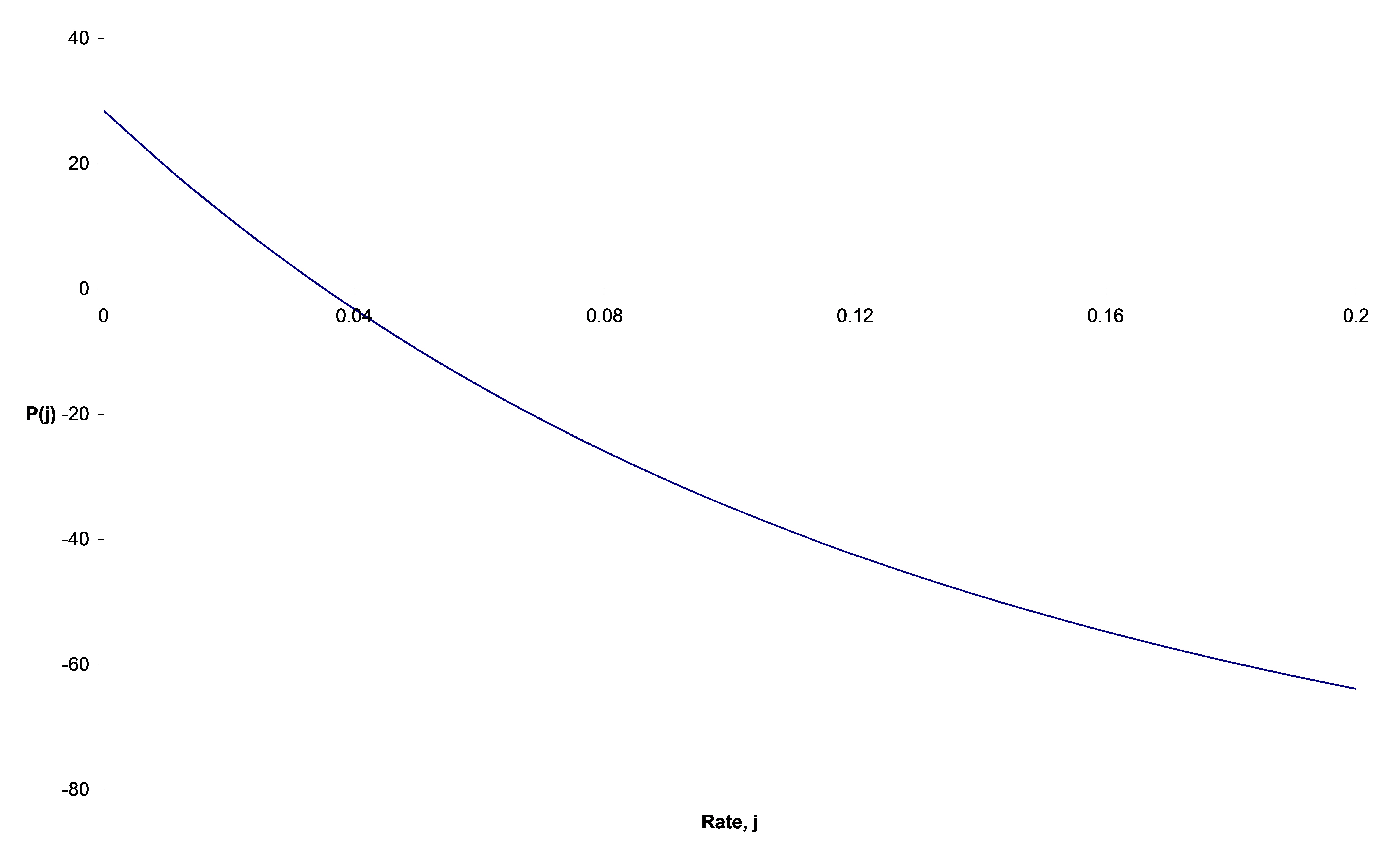
The plot below shows \(P(j)\) over a much wider range of values for \(j\).
It is clear that the assumption of linearity may be reasonable over narrow intervals, but not wide ones.
Hence we assume
\begin{align*} P(j)=\alpha +\beta j, \quad j\in[3.5\%, 3.6\%] \end{align*}
The solution to the equation \(P(j)=0\) is therefore \(j=-\alpha /\beta\)
We use the results in Step 2 to find the values of \(\alpha\) and \(\beta\). We get two simultaneous equations, as follows:
\begin{eqnarray*} \alpha +0.035\beta &=&0.2185, \\ \alpha +0.036\beta &=&-0.4732. \end{eqnarray*}
Solving these equations gives \(\beta =-691.7\) and \(\alpha =24.428\).
Therefore our approximation to the semi-annual yield is
\begin{align*} j=\frac{-\alpha }{\beta }=\frac{-24.428}{-691.7}=3.532\%. \end{align*}
Summary #
Wrapping up:
- Given that our yield per half year is 3.532%, the nominal
per annum yield convertible half-yearly is
\(7.064\%\). - If the purchasing price is larger than the face value (e.g.
\(P=101.50>100\)), then the yield is lower than the coupon rate\((7.064\% <7.5\% )\) - If the purchasing price is smaller than the face value (e.g.$P=99<100$ ), then the yield
\((3.90\%\times 2=7.8\% )\)is higher than the coupon rate 7.5%. - If Price is equal to the Face Value (100), then yield=7.5%=coupon rate.
The effect of tax #
Tax matters #
- All individuals and for-profit organisations are subject to tax on income and capital gains.
- In the context of bonds, coupons are income.
- The difference between the price paid and the capital payment at the maturity date is a capital gain (or loss).
- For example:
- Suppose a bond pays an annual coupon of $8 per $100 nominal.
- Suppose that an investor is subject to income tax at 25%.
- Assuming that coupons are paid net of tax, the investor would receive $6 per $100 nominal, i.e. 75% of $8.
- To complicate matters, individuals face a different tax rate, depending on their level of income. This may be uncertain when making decisions.
Example 9 #
- A government is about to issue a bond which has a term of 25 years and pays coupons half-yearly at 6% per $100 nominal.
- An investor is subject to income tax at 30%.
- What price should this investor pay per $100 nominal at issue to secure a yield of 5% per annum effective after tax?
Solution:
- The price is the present value at 5% per annum effective of the net of tax payments that the investor will receive.
- The investor receives an annuity of
\(0.7 \times 6=4.2\)dollars per annum (payable half-yearly). - Thus, the price is
\begin{eqnarray*} &&4.2a_{\angl{25}}^{(2)}+100v^{25}\qquad @5\%\\ &=&89.46 \end{eqnarray*}since\(a_{\angl{25}}^{(2)}=14.26797\).
Example 10 #
- Sophie has $100,000 in cash to invest over the next 10 years.
- She can either:
- leave the money in her home loan offset account, with full offset of her current (variable) rate of 3.2%; or
- invest the money in a 10 year bond from a reputable Australian company, at a coupon rate of 4%.
What should Sophie do?
References #
Atkinson, M. E., and David C. M. Dickson. 2011. An Introduction to Actuarial Studies. 2nd ed. Edward Elgar.